• Categories
• Cimentación profunda
• Roca (Geología)
• Mecánica de sólidos
• Mecánica Continua
• Infraestructura

Citation preview

GEOTECHNICAL ENGINEERING ,\ I'r .• (uc.d Prubkm SUIVlIH,:' Appru.uh

DWD IOC'" DOO

GEOTEC:HNICAL EN G INI~ERINCA Practical Problem Solving Approach

N. Sivakugan I Hraja M. Das

J.RO~;) · ....

PUBLI S HI NG

l~

Copyright C> 2010 by J. Ross Publishing, Inc. ISBN-13: 978-1-60427-016-7 Printed and bound in the U.S.A. Printed on acid-free paper

library of Congress Cataloging-in - Publication Data Sivakugan, Nagaratnam . 1956Geotechnical engineering: a practical problem solving approach I by Nagaratnam Sivakugan and Braja M. Das. p.cm. Includes bibliographical references an,d index. ISBN 978- 1-60427-016-7 (pbk. : alk. paper) l. Soil mechanics. 2. Foundat ions. 3. Earthwork. 1. Das. Braja M .• TA710.S5362oo9 624. 1'5 136- dc22

2009032547 This publication contai ns information obtained from authentic and highly regarded sources. Reprinted material is used with permission, and sources are indicated. Reasonable effort has been made to publish reliable data and information, but the author and the publisher cannol assume responsibility for the validity of all materials or fo r Ihe consequences of their use. All rights reserved. Neither this publication nor any part thereof may be reproduced, stored in a retrieval system. or transmitted in any form or by any means, cleCironic, mechanical, photocopying, recording or otherwise, without the prior written permission of the publisher. The copyright owne r's consent does not extend to copying for general distribution for promotion, for creating new works, or for resale. Speci fi c permission must be obtained from J. Ross Publishing for such pur poses. Di rect all inquiries to J. Ross Publishing, Inc.. 5765 N. Andrews Way, Fori Lauderdale, FL 33309. Phone: (~51) 727-'3333 Fax: (561) 892-0700

Web: www.jrosspub.com

To our parents. teachers, and wives

iii

Contents Preface ................................................................................................................................................................... ix Aboul the Authors................................................................................................................................................ xi WAVT,.t ...•....................................................................... ..................................................................................... xiii

Chapter I Introduction ........................... ....................................... ... ..... ......... ..... ................................ 1 1.1 General ............... ,......................... ................... ............................ ............ .......................................... .............. 1 1.2 Soils.................. ............................ ............... .............................. .................. ....... ...... ... ... .............. ..... ........ 1 1.3 Applications ....................................................................................................... ..................... .... ...... .. .... ....... . 3 1.4 Soil Testing ......................................................................................................................................... .......... .. . 3 1.5 Geotechnical Literature ................. ................................................................................................... ............. 4 1.6 Numerical Modeling .. ............................................................................................................................... .... 6 Review Exercises .................................................................................. ...... ............................................................ 8 Chapter 2 Phase Relatio ns ................................................................................................. .. .. ..... ....... 11 2. 1 Introduction ......................................................................................................................... ......... ... ....... ...... 11 2.2 Definitions ... ..... ........ .. .................. ......................................................................................................... ..... 11 2.3 Phase Relations ........... ................................................................................. .................................... ............ 13 Worked Examples .. .......... .. ......................................... ............ ............ ... ..................... .. .................................. . 16 Review Exercises.... ..... .... .. .............. ................................................ .......................................................... 22 Cha pter 3 Soil Classification ............................................................... .......................... ..... ............... 2 7 3. 1 Introduction ................................. ........... ...................................................................................................... 27 3.2 Coarse-G rained Soi ls ............................................................................................................................ .... ... 27 3.3 Fine-Grained Soils ................................................................................................................................. ...... 32 3.4 Soil Classification ............................................................................................................... .. ............. ..... ...... 37 \oVorked Exanlpies ....... .. ........ ............................................................................................... ,.............................. 41 Review Exercises.......................................... ............... .................................................................. ........ ............... 44 Chapter 4 Compaction ................. .. ............ ......... ... .... ... .... ... .... ................. .. .... ...... .. ........................... 49 4.1 Introduction ................................................................................................................................................. .49 4,2 Variables in Conlpaction ....................................................... ..... ............................................................... 50 4.3 Laboratory Tests ........................................................................................................................................... 52 4.4 Field Compaction. Specificat io n, and Control .. .................................. ........... ,............ , ..... 55 \oVorked Examples .......................................................................................................................................... ... ... 59 Review Exercises ................ .... .... .... ............................................................................................................... ..... 62

v

vi Contents

Chapte r 5 Effective Stress, Total Stress, and Pore -Water Pressure ... .......................... ....... ...............65 5.1 Introduction ............... ................... ................ ......... .... .... .... .. ..................... .................................... 65 5.2 Effect ive Stress Principle.................... ... .... ... ..................... ... .............................. .......... 65 5.3 Vertical Norma l Stresses Due to O verburden ..... ............ ..... .... ................................... ........................... 66 5.4 Capillary Effects in Soils ............... .... .. .. .................... ...... ................................ .. ... ... ... 68 vVorked Examples ............... .... ... ..... ... ... .. ... ...... ... ... ........ .. ... .... ................. ... .... ... ... ... .. ......... .. ................... .. .... ...... 70 Review Exercises .. ................... .... ...... ............................. ............................. ........... ............ ..... ... ....... .................. 71 Chapter 6 Permeability a nd Seepage ........................................ ............................................... .......... 73 6. 1 Introduction ................ ................. ......................... .................. ............. ....... ............. ..... ............ .... .. ........... .. 73 6.2 Bernoulli's Equation ............................................. .. ........ ...... ... ..... ....... .................... ...................... .. ........... .. 73 ... ..... 76 6.3 Darcy's Law .... ..... ............ .. . .... ............ .. ... ...... ... ..... ...... ............................. .... ..... ... ...................... 6.4 Labo ratory and fi eld Permeability Tests .......... ........ .... .... ..... ................ .... .... ...................... ...... .. 77 6.5 Stresses in Soils D ue to Plow ................ ............. ... ... ...... ... ................. ... ...... ..... 81 6.6 Seepage ......................... ... ............... .. ............... ....... 82 ... ........................... .............................................. ....... 86 6.7 Design of Granular Filters ......... ... ...... ...... .. 6.8 Equivalent Permeabilities fo r O ne -di mensional Flow ........................... .................. ..... .. .................. ...... 87 6.9 Seepage An alysis Using SEEP/ llll .. ......................................... ................... ..... ...... ........... ........ .............. .... 89 'vVorked Examples ................................................................................................................................ .................94 Review Exercises .. ... ..... .. ....... ....... ......... ..... ................... ._........ . .... ... ... ............ .... ........................ .......... 103 Chapter 7 Vertical Str esses Beneath I..oaded Areas...........•.•....•......•.... ......... ,.... ............_................ 115 7. 1 Introd uction ............................................ ..... ............. .......... ........................................................... .. .... .... ... 11 5 7.2 Stresses Due to Point Loads ......... .. .... ... ........... .. ..... ... ... ..... ................................. ...... ................. ............ 116 7.3 Stresses Due to Line Loads ..... .. .. ........ ... .... ..... ...... .... ...... ......... .. ... ...... .... .......... ... ....... ........... ...... ....... ...... 11 8 7.4 Stresses Under the Corner of a Uniform Rectangular Load.............. .......... .... .. ... . 11 8 7.5 2: 1 Distribution Method .............. ............................................................. .............. ... ... ..... ...... ... 123 7.6 Pressure Isobars Under Flexible Uniform Loads ............ ..................... . ........ ..... ..... .... 124 7.7 Newmark's CharL ...... ..... ........ ........................... . .... .......... ... ......................... ............ ............. ... 124 7.8 Stress Computations Using SIGM A/W ......... ... ............... ................................ .. ........... 129 Worked Examples ............... . .......................... .. .......... 133 Review Exercises .. ................................... ....................... .. ................... .... . ......... ............. ................. ..... 136 C hapter 8 Consolidation ............................................................................ ...................................... 139 8.1 Introduction .. ......... ... .................................................................. ... ........... .... .. .... ...... ...... ...................... .. .. 139 8.2 One· dimensional Consolidation ................ .,........ .... ............................... ... ................... ................ .......... 140 8.3 Consolida tion Test ........ ................ ................ ......... .................................. ............

... ... .. .................. ... 143

8.4 Computation of Final Consolidation Settlement ................................... ............ ...... ........ ....... ...... ..... ... 150 8.5 Time Rate of Consolidatio n ...... .......... ............................... ...... ............... ............... ............. ...... ............... 153 8.6 Secondary Compression ...................... ................................... ... ... ... ...... ...................................... ............ 159 Worked Examples................... .. ........ ........... ... . ....... ............. ............... ....... .......... ............ 165 .... ..... .... 175 Review Exercises.. ...... .............................. ... .................... ........ .... ... ........................ ................

Contents vii

Chapter9 Shear Strength ...................................... ........... .......... .. .................................................... 181 9. 1 Introduction ............................................................................................................................................. 18 1 9.2 Mohr Cirdes ............................................................................................................................................. 18 1 9.3 Mohr-Coulomb Failure Criterion ...................... _........................ .......... ................................................ 186 9.4 A Common Loading Situation .................. .... ..... . ........................... ........ ............................................... 187 9.5 Mohr Circles and f ailure Envelopes in Terms of fJ and fJ' .............. ........... .. ................................ ..... 190 9.6 Drained and Undrain ed Loading Situations.... .... .. .. ... .. ........ .. .... ....... ...... ................................... 191 9.7 Triaxial Test .................................................... .......... ... ... .... ........ .. .. ..................... ..... .......... .. . ........ 193 9.8 Direct Shear Test ...................... ......... ... ... ............. .. .. ........... ...... ...... ........ .... ....... .... ..... ... ................. ...... 200 9.9 Skempton's Pore Pressure Parameters .. ...................................... ......... .... .. ... ..... .... ................................ 202 9. 10 0 1 - OJ Relationship at Failu re ................................................................................................................ 205 9. 11 Stress Paths ........................................................................................ ....................................................... 206 \'\Iorked Examples ........................ ......... .... ........... .. .. ..... ............... ... .. .... .... .. ...................................... .. .. 21 0 Review Exercises ................................ ..... .. .. ... ................. ................ ... .. ............ ..... .......................... ............ ...... 21 7 C hapter 10 Lateral Earth PressuTcs ................................................................................................. 225 10.1 Introduction ..... .. ..... ..................... ......... ...... ............................................ ....... .. .... ..... ....... .. ... ................... 225 10.2 At-rest State .................................. ............................................................. ........... ... ... ... ............ ...... ......... 226 10.3 Ranki ne's Earth Pressure Theory.................................................. ...................... ................................... 230 10.4 Coulomb's Earth Pressure Theory ......................................................................................................... 237 vVorked Examples .................. ................................................................ ............................................................ 240 Review Exercises .......................................... ...................................................................................................... 246 Chapter II Site Investigation .................................. .. ..................... .............. ... ..... .......................... 251 11 .1 Introduction ....................................................................................... ....... ....................................... ..... ... 251 11 .2 Drilling and Sampling ..................................................... ... ............... .... ............................ ... ... ....... ......... 253 11 .3 In Situ Tests............................................ ............................... .................. ................ .................................. 257 11.4 Laboratory Tests ....... ...... .. ...... .. ....... .. ... .............................................. ... ........................................ ........... 276 11 .5 Site Invest igation Report ...................................... ....... ... ... .... .. ..... ....................................................... .... 276 "V\'orked Examples ...................... .... ... ... .. .. ...... ... ....................................................................................... ... ... .... 280 Review Exercises ... .......... ................................................ ......................................................................... ... ... .... 283 Chapter 12 Shallow Foundalions .......................... ................................................... ........ .............. 289 12.1 Introduction ............. ....... .... ... .................................................................................................................. 289 ............. ................ .................... ........... ..................................... 290 12.2 Design Criteria.......... .. .... ..... 12. 3 Bearing Capacity of a Shallow foundation ........ .......................................... .. ... .......... ......................... 291 12.4 Pressure Distributions Beneath Eccentrically Loaded Footings ................... ............................. ...... 301 12.5 Introduction to Raft Foundation Design ........................ ...................................................... ........... ...304 12.6 Settlement in a Gran ular Soi l ..... .. .............................. ............................ .. .. .. ........... ............................... 310 12.7 Settlenlent in a Cohesive Soil ....................................................................................................... ... ... .... 3 19 \Vorked ExampJes .............................................................................................................................................. 325 Review Exercises ............................. .. .. .......... .. ... ................................................................................................ 334

viii Contents

Chapter 13 Deep Foundations ...................... ................................................................................. 341 13.1 Introduction.. ........................ ................. ...... ............................................................. ...... 34 1 13.2 Pile Materials ............................................ .. .................... .................................... ... .... .. ... .342 13.3 Pile Install ation ..... .................. ..... ...... .... ..................................................................... 345 .................. ..................................... .. .. 347 13.4 Load Carrying Capacity of a Pile- Static Analysis. 13.5 Pile· Driving Formulae .................................................................................. .... ..... ................ .. 354 13.6 Pile Load Test ..................................... .......... ................................................... ......................................... 355 .............. ...... ... 357 13.7 Sett lement ofa Pile.................................................................................. ...... .... 13.8 Pile Group ................................................................................................ ....... ...... ............. ....................... 361 Worked Examples ........................................................................................................... .. ... .............................. 365 Review Exercises................................................................................................................................................ 373 C hapter 14 Earth Retaining Structures ........................................................................................... 377 14.1 Introduction ............. .................. .... ............. ... ................................................................ ...... 377 14.2 Design of Retaining Walls ................ .......... .... ................................................. .. .. .... 379 14.3 Cantilever Sheet Piles ............................ .............. "................................................................................ 385 14.4 Anchored Sheet Piles .............. .. .............................................................................. ... ..... .......... 395 14.5 Braced Excavations.................................................................................. ................................... 399 Worked Examples ............................................................................................................................................... 404 Review Exercises.. ............... ............................................................................................ ..... .............................. 415 Chapter 15 Slope Stability .......... ......................................................................................................421 15.1 Introduction ......................................... ......................................................................................... .. .... ...... 421 15.2 Slope Failure and Safety Factor .. ......................... ......... ..... ... ................. ... ........ .................................... 422 15.3 Stability of Homogeneous Undrained Slopes ..................... .. ........................ ....................................... 423 15.4 Taylur's Stability Charts fur e '1>' Soils ........ ..... .......... .... .............. .. .... ....................... 427 15.5 Infinite Slopes .......... ............. ..... ... ........ ............... .... ........... ...... .. .......... .. .......... ...................... 129 15.6 Method of Slices............................ ......... ............... ................... ..................................... ....... .. 432 15.7 Stability Analysis Using SLOPE/W..................... ................................................ ..................... .435 \""orked Examples ..................................................................................................................................... ......... 443 Review Exercises .......................................................... .. ............ .... ....................................................... .. .......... 449 Chapter 16 Vibrations of Foundations ............................................................................................. 453 16. 1 Introduction ........................ .............. .......... ... ..................................................... 453 16.2 Vibration Theory- General ........................................................................ ... .... ....................... .............. 454 16.3 Shear Modulus and Poisso n's Ratio ...... ............... ..................................................... ............................. .463 16.4 Vertical Vib ration of ~oundations - An alog Solution .................................. .. .................................. 165

16.5 Rocking Vibration of f oundat ions ...................... ............................................... .............. ........ .... ..... .... .469 16.6 Sliding Vibration of Foundations ........................ ... ........................................... ......... ...... ....... .475 16.7 Torsional Vibration of Foundations ................................................................................... ..... ..... ....... ..478 Review Exerdses ........................... .... ............................... .............. ............... ............... ................. ..................... 483 Index ........................................................................ ............. ...................... ................ ....................... 487

Preface We both have been quite successful as geotechnical engineering teachers. In Geotechnical Engineering: A Practical Problem Solving Approach, we have tried to cover every major geotechnical topic in the simplest way possible. We have adopted a hands-on approach with a strong, practical bias. You wiU learn the material through several worked examples that take geotechnical enginee ring principles and apply them to realistic problems that you are likely to encounter in real-life field situations. This is OUf attempt to wr:ite a straightforward, no-nonsense, geotechni cal engineering textbook that will appeal to a new generation of students. This is said with no d isrespect to the variety of geotechnical engineering textbooks already available-each serves a purpose. We have used a few symbols to facilitate quick referencing and to call your at tention to key concepts. Th is symbol appears at the end of a chapter wherever it is necessary to emphasize a particular point and your need to understand it. There are a few thoughtfully selected review exercises at the end of each chapter, and answers are given whenever possible. Remember, when you practice as a professional engineer you will not get to see the solutions! You will simply design with confidence and have it checked by a colleague. The degree of difficulty increases with each review exercise. The symbol shown here appears beside the most challenging problems. We also try to nurture the habit of self-learning through exercises that relate to topics not covered in this book. Here, you are expected to surf the Web; or even better, refer to library books. The knowledge obtained from both the reseal-ch activity and the material itself will complement th e lIIah::rial from this book and is an integral part of learning. Such research -type questions are identified by the symbol shown here. Today, the www is at your fingertips, so this should not be a problem. There are many dedicated Web sites for geotechnical re-

~

~

~indel'

sources and reference materials (e.g., Center for Integrating Information on Geoengi neer-

ing at http://www.geoengineer.org). Give proper references for research-type questions in your short essays. Sites like Wikipedia (http://en .wikipedia.org) and YouTube (http:lh."""", .youtube.com) can provide useful information induding images and video dips. To obtain the best references, you must go to the library and condu ct a proper literature search using appro priate key words. ix

x Preface

We have included eight quizzes to test your comprehension. These are closed book quizzes that should be completed within the specified times. They are designed to make you think and show you what you have missed. The site investigation chapter has a slightly different layout. The nature of this topic is quite descriptive and less reliant on problem solving. It is good to have a clear idea of what the different in situ testing devices look like. For this reason, we have included several quality photographs. Thl;: purpose of the site investigation exercise is to derive the soil parameters from the in situ lest data. A wide range of empirical correlations that are used in practice are summarized in this chapler. Tests are included that are rarely covered in traditional textbooks-such as the borehole shear test and the Kostepped blade test- and are fo llowed by review questions that encourage the reader to review other sources of literature and hence nurture the habit of research. Foundation Engineering is one of the main areas of geotechnical engineering; therefore, considerable effort was directed toward Chapters 12 and 13, which cover the topics of bearing capacity and settlements of shallow and deep foun dations. This is not a place for us to document everything we know in geotechnical engineering. We realize that this is your first geotechnical engineering book and have endeavored to give sufficient breadth and depth covering all major topics in soil mechanics and foundation engineering. A free DVD containing the Studem Edition of GeoStudio is included with th is book It is a powerful software suite that can be used for solving a wide range of geotechnical problems and is a useful comp l~menl to traditional learning. We are grateful to Mr. Paul Bryden and the GeoStudio team for their advice and support. We are grateful to the follOWing people who have contributed either by reviewing chapters from the book and providing suggestions for improvement: Dr. Jay Ameratunga, Coffey Geotechnics; Ms. Julie Lovisa, James Cook University; Kirralee Rankine, Golder Associates; and Shailesh Singh, Coffey Geotechnics; or by providing photographs or data: Dr. Jay Ameratunga, Coffey Geotechnics; Mr. Mark Arnold, Douglas Partners; Mr. Martyn Ellis, PMC. UK; Professor Robin Fell, University of New South Wales; Dr. Chris Haberfleld. Golder Associates; Professor Silvano Marchetti, University of LAquila, Italy; Dr. Kandiah Pirapakaran, Coffey Geotechnics; Dr. Kirralee Rankine, Golder Associates; Dr. Kelda Rankine. Golder Associates; Dr. Ajanta Sachan. lIT Kanpur, India; Mr. Leonard Sands, Venezuela; Dr. Shailesh Singh, Coffey Geotechnics; Mr. Bruce Stewart, Douglas Partners; Professor David White, Iowa State University. We wish to thank Mrs. Janice Das and Mrs. Rohini Sivakugan. who provided manuscript preparation and proofreading assistance. Finally, we wish to thank Mr. Tim Pletscher of J. Ross Publishing for his prompt response to all our .questions and for his valuable contributions at various stages. N. Sivakugan and B. M. Das

About the Authors Dr. Nagaratnam Sivakugan is an Associate Professor and Head of Civil and Environmental Eng ineering at the School of Engineering and Physical Sciences, James Cook UniversityAustralia. He graduated from the University of.Peradeniya-Sri Lanka, with First Class Honours and received his MSCE and PhD from Purdue U niversity. As a chartered professional engineer and registered professional engineer of Queensland, he does substa ntial consulting work for geotechnical and mining compan ies th roughout Australia and the world. He is a FeUow of Engineers, Australia . Or. Sivakugan has supervised eight PhD candidates to completion and has published morc than SO scien tific and technica l papers in refereed international journals, and SO more in refereed international conference p roceedings. He serves on the editorial board of the international Journal of Geotechnical Engineering (lIGE) and is an active reviewer for morc than IO international journals. In 2000, he developed a suite of fully animated Geotechnical PowerPoinl slirJcshows th at are now used worldwide as an effective teach ing and learning tool. An updated version is available for free downloads at http://v{Ww.jrosspub. com. Dr. Braja M. Das, Professor and Dean Emerit us, California State University-Sacramento, is presently a geotechn ica l consulting engineer in the state of Nevada. He earned his MS in civil engi nee ring from the University ofIowa and his PhD in geotechnical engineering from the Uni versity of Wisconsin- Madison. He is a Fellow of the American Society of Civil Engineers and is a registered professional engineer. He is the author of several geotechnical engineeri ng texts and reference books including Principles of Geotechnical Engineering, Principles of Foundation Engineering, Pundamentais of Geotechnical Engineering, Introduction to Geotechnical Engineering, Prim.:iples uf Sui! Dynamics, Shallow Foundations: Bearing Capacity and Settlement, Advanced Soil Mechanics. Earth Anchors. and Theoretical Foundation Engineering. Dr. Das has served on the editorial boards of several international jou rnals and is currently the editor in ch ief of the International Journal of Geotechnical Engineering. He has authored more than 250 technical papers in the area of geotechnical engineering.

xi

VRI ~ This book has free matBfial available for download from the

Web Added Value'" resource center at www.jrosspub.com

At J. Ross Publishing we are committed to providing tadar's professional with practical, hands-on tools that enhance the learning experience and give readers an opportunity to apply what they have learned. That is why we offer free ancillary materials available for download on this book and all participating Web Added Vaiue- publications. These online resources may include interactive versions of material that appears in the book or supplemental templates, worksheets, models, plans, case studies, proposals, spreadsheets, and assessment tools, among other lhings. W henever you ~cc the WA V N symbol in any of OUf publications, it means bonus materials accompany the book and are available from the \'\feb Added Val u e~ Download Resource Center at www.jrosspub .com. Downloads for Geotechnical Engineering: A Practical Problem Solvillg Approach include PowerPoint slides to assist in classroom instruction and learning.

Introduction

1

1.1 GENERAL What is Geotechnical Engineering? The term geo means earth or soil. There are many words that begin with geo-geology, geodesy, geography, and geomorphology to name a few. They all have something to do with the earth. Geotechnical engineering deals with the engineering aspec ts of soils and rocks, sometimes known as geomaterials. It is a relatively young d iscipline that would not have been part of the curriculum in the earlier pari of the last century. The designs of every building, service, and infrastruc ture fac ility bui lt on the ground must give due consideration to the engineering behavior of the underlying soil and rock to ensure that it performs sat isfactorily during its design life. A good understanding of engineering geology wiJi strengthen your skills as a geotechnical engineer. Mechanics is the physical science that deals with fo rces and equilibriu m, and is covered in subjects like Engineering Mechanics, Strength of Materials, or Mechanics of Materials. In Soil Mechanics and Rock Mechanics, we apply these principles to soils and rocks respectively. Pioneeri ng work in geotechnical engineeri ng ·was carried out by Karl Terlagh i (1882- 1963), acknowledged as the father of soil mechanics and author of Erdbaumechanik auf bodenphysikalischer grund/age (1925), the first textbook on the subject. Foundat ion Engineering is the applicat ion of the soil mech anics pri nciples to design earth and earth-sup ported st ructures such as fo undatio ns, reta ining st ruc tures, dams, etc. Traditional geotechn ical engineer ing, which is also called geomechanics or geoengineering, includes soil mechanics and fo un dation engineering. The escalat ion of hum an interference with the environment and the subsequent need to address new problems has created a need for a new branch of engineering that will deal with h aza rdous waste disposal, landfi lls, ground water contamination, potential acid su lphate soils, etc. This bra nch is called enviromnental geomechanics or geoenviro ll1nental engineering.

1.2 SOilS Soils are formed over thousands of years through the weathering of parent rocks, which can be igneous, sedimentary, or metamorphic rocks. Igneous rocks (e.g., granite) are formed by the cooling of magma (underground) or lava (above the ground). Sedimentary rocks (e.g., li mestone,

2 Geotechnical Engineering

shale) are formed by gradual deposition of fine soil grains over a long period. Metamorph ic rocks (e.g., marble) are formed by altering igneous or sedimentary rocks by pressure or temperature, or both. Soils are primarily of two types: residual or transported. Residual soils remain at the location of their geologie origi n when they are formed by weatheri ng of the parent rock. When the weath ered soils are transported by glacie r, wi nd, water, or gravity and are deposited away from th ei r geologic origin, they are call ed transported soils. Depending on the geologic agent involved in the transportation process, the soil derives its special name: glacier-glacial; wind-aeolian; sea - marine; lake-lacustrine; river-alluvial; gravity-colluvial. Human beings also can act as the transporting agents in the soil formation process, and the soil thus form ed is called a fill. Soils are quite different from other engineering materials, which makes them interesting and at the same time challenging. Presence of water within the voids fu rther complicates the picture. Table 1.1 compares soils with other engi neerin g materials such as steel. We often simpli fy the problem so that it can be solved using soil mechanics prinCiples. Sometimes soil is assumed to be a homogeneous isotro pic cl astic continuum , which is far from reality. Nevertheless, such approximations enable us to develop simple th eories and arrive at some solutions that may be approximate. Depending on the quality of the data and the degree of simpli fication, appropriate safety factors are used. Geotechnical engin eering is a sc ience, but its practice is an art. There is a lot of judgment involved in the profession. The same data can be inter preted in different ways. When there are limited data available, it beco mes necessary to make assumptions. ConSid eri ng the simplifica tions in the geotechn ical engineering fundamentals, uncertainty, and scatter in the data, it may no t always make sense to calculate every thing to two decimal places. All these make th e fiel d of geotechnica l engin eer ing qui te different from othe r engi nee rin g disciplines. Table 1.1 Soils vs. other engineering materials Soils

Others (e.g., steel)

1. Particulate medium - consists of grains

Continuous medium - a continuum

2. Three phases-solid grains, water, and air

Single phase

3. Heterogeneous-high degree of variabHity

Homogeneous

4. High degree of anisotropy

Mostly isotropic'

5. No tensile strength

Significant tensile strength

6. Fails mainly in shear

Fails in compression, tension, or shear

'Isotroplc - same prope!ty in all directions

Introduction 3

1.3 APPLICATIONS Geotechnical engineering applications include foun dations, retaining walls, dams, sheet piles, braced excavations. reinforced earth , slope stability, and groun d improvement. foundations such as footings or piles are used to support buildings and transfer the loads from the superstructure to the underlying soils. Retaining walls are used to provide lateral support and maintai n stability between two different ground levels. Sheet piles are conlinuous impervious walls thal are made by driving interlocking sections into the ground. They are useful in dewatering work. Braced excavation involves bracing and supporting the walls of a narrow trench, which may be required for burying a pipel ine. Lately> geosynthetics are becoming inc reasingly popular for reinforcing soils in an attempt to improve the stability of footings, retaining walls, etc. When working with natural or man-made slopes, it is necessary to ensure their stability. The geolechnical characteristics of weak ground are often improved by ground improvement techniques such as compaction, etc. Figure 1.1a shows a soil nailing operation where a reinforcement bar is placed in a drill hole and surrounded with concrete to provide stability to the neighboring soil. Figure 1.1 b shows the haipu Dam in Brazil, the largest hydroelectric facility in the world. Figure l.I c shows trealcd timber piles. Figure l.ld shows steel sheet piles being driven into the ground. Figure l.Ie shows a gabion wall that consists of wire mesh cages filled with stones. Figure I.If shows a containment wall built in the sea for dumping dredged spoils in Brisbane, Australia.

1.4 SOIL TESTING Prior to any design or construclion , it is necessar y to understand the soi l con ditions at the sit e. Figure 1.2a shows a trial pit that has been made llsing a backhoe. Tt gives a clear idea of what is lying beneath the ground. but only to a depth of 5 m or less. The first 2 m of the pit shown in the figure are clays that are followed by sands at the bottom. Samples can be taken from these trial pits for furt her study in the laboratory. Figure 1.2b shows the drill rig set up on a barge for some offshore site investigation. To access soils at larger depths, boreholes are made usi ng drill rigs (Figure 1.2c) from which samples can be collected. 'rhe boreholes are typically 75 mm in diameter and can extend to depths exceeding 50 m. In addition to taking samples from boreholes and trial pits, it is quite common to carry out some in situ or field tests within or outside the boreholes. The most common in situ test is a penetration test (e.g., standard penetration test, cone penetration test) where a probe is. pushed into the ground, and the resistance to penetration is measured. The penetration resistance can be used to identify the soil type and estimate the soil strength and stiffness.

4 Geotechnica! Engineering

(a)

(b)

(e)

(d)

(e)

(Q

Figure 1.1 Geotechnical applications: (a) soil nailing (b) Itaipu Dam (c) timber pi les (d) sheet piles (e) gabion wall (Courtesy of Dr. ~(irra l ee Rankine, Golder Associates) (f) sea wall to con tain dredged spoils

1.5 GEOTECHNICAL LITERATURE Some of the early geotechn ical engineering textbooks were written by Terzaghi ( 1943), Terzaghi and Peck (I948, I % 7), Taylor (1948), Peck et a!. (I 974), and Lambe and Wh itman (1979). "I hey are cl assics and will always have their place. W hile the content and layout may not appeal to

Introduction 5

(a)

(e) (b)

Figure 1.2 Soillesting: (a) a trial pit (Courtesy of Dr. Shailesh Singh) (b) drill rig mounted on a barge (Courtesy of Dr. Kelda Rankine, Gol!jer Associates) (e) a drill rig (Courtesy of Mr. Bruce Stewart, Douglas Partners)

the present generation, they serve as useful referen ces. Geotechnical journals provide reports on recent developments and any innovative, global research that is being carried out on geotechn ical topics. Proceedings of conferences can also be a good reference source. Through universities and research organizations. some of the literature can be accessed online or ordered through an interlibrary loan. There are still those who do not place all their work on the Web, so you may not find everything you need simply by surfing. Nevertheless, there are a few dedicated geotech nical Web sites that have good literature, images, and videos. When writing an essay or report, it is a good practice to credit the source when referring to someone else's work, including th e data. A common practice is to include in parentheses both the name of the author or authors and the year of the publication. At the end of the report, include a complete list of references in alphabetical order. Each item listed should include the nam es of the authors with their in itials, the year of the publication, the title of the publication, the publishing company, the location of the publisher, and the page numbers. The style of referencing and listing d iffers between publications. In th is book (See References), we have followed the style adapted by the Amer ican Society of Civil Engineers (ASCE) .

6 Geotechnical Engineering

Professional engineers often have a modest collection of handbooks and design aids in their libraries. These include the Canadian Foundation Engineering Manual (2006), the Naval Facility Design Mallual (U.S. Navy 1971 ), and the design manuals published by u.s. Army Corps of Engineers. These handbooks are written mainly for practicing engineers and will have limited coverage of the theoretical developments and fu ndamentals.

1.6 NUMERICAL MODELING Numerical modeling involves finite element or finite difference techniques that are implemented on micro or mainframe computers. Here, the soil is often represented as a continuum with an appropriate constitutive model (e.g., linear elastic material obeying Hooke's law) and boundary conditions. The constitutive model specifies how the material deforms when subjected to specific loading. The boundary conditions define the loadi ng and displacements at the boundaries. A problem without boundary conditions cannot be solved; the boundary conditions make the solution unique. Figure 1.3 shows a coarse mesh for an embankment underlain by Iwo different soil layers. Due to symmetry, only the right half of the problem is analyzed, thus saving computational time. Making the mesh finer will result in a bdter solution, but will increase computational time. The bottom and right boundaries are selected after some trials to ensu re that the displacements are negligible and that the stresses remain unaffected by the em bankment loading. The model geometry is discretized into hundreds or thousands of elements, each element having three or four nodes. Equations relating loads and displacements are written for every node, and the resulting simultaneous equations are solved to determine the unknowns. ABAQUS, PLAXIS, FLAC, and GeoStudio 2007 are some of the popular software packages that are being used in geotechnical modeling wo rldwide. '10 give you a taste of numer ical modeling, we have included a free DVD containing the Student Edition of GeoStudio 2007, a software suite developed by GEO-SLOPE Imemationaf (http:/hV\vw.geo-slope.com) to perform numer ical modeling of geotechnical and geoenviron mental problems. It is quite popular worldwide and is being used in more than 100 countries; not only in universities, but also in professional practices by consulting engineers. It includes eight stand -alone software modules: SLOPEIW (slope stability), SEEPIW (seepage), SIGMAIW (stresses and defo rmati ons), QUAKEIW (dynamic loadings), TEMPIW (geothermal), CTRANI W (contaminant transport ), AIRlW (airflow), Hnd VADOSEIW (vadose zone and soil cove r), which are integrated Lu work wiLh each oLher. For example, the uutput fro m one program can be imported into another as input. There are tutorial movies that are downloadable from the Web site. Press FJ for help. You can subscribe to their free month ly electronic newsletter, Direct Cot/tact, which has some useful tips that will come in handy when using these programs. The GeoStudio 2007 Student Edition DVD induded wiLh Lhis book cOll lains all eight programs with limited features (e.g., 3 materials, 10 regions, and 500 elements, when used with

Introduction 7

~~~~~~i;Emb_a"_'_

ODIC I

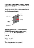
Per minute: V, _ 400 liters VI'" y m~

1.5m 15m

I•

Y.. = 18.7 kNlm3

Volum e of soil to be removed = (1 .5)(15)(200) = 4500 m J . In situ unit weight (saturated) = 18.7 kN/m l .

+ S = (0.124)(2.75) 1(0.580) = 0.588 or 58.8% G, 10. A sample of an irregular lump of saturated day with a mass of 605.2 g was coated with wax. The total mass of the coated lump was 614.2 g. The volume of the coated lump was determined to be 311 cm l by the water displacement method as used in Worked Example 9. After carefully removing the wax, the lump of day was oven dried to a dry mass of 479.2 g. The specific gravity of the wax is 0.90. Determine the water content, dry unit weight, and the specific gravity of the soil gr-ains. Solution:

M, = 605.2 g, M, = 479.2 g -t M", = 126.0 g, V", = 126 cm~ and w = 26.3% Mw.. = 614 .2 - 605.2 = 9.0 g --> V.., = 9.010.9 = 10 em' V""ilg"'in, = 3 11 - 126 - 10 = 175 cm l -t G, = 479 .2/175 = 2.74 Pd = 479.2/(175 + 126) = 1.592 g/cm' --> 'Yd = 1.592 X 9.81 = 15.62 kN/m ' II. A series of experiments are being conducted in a laboratory where fly ash (G, = 2.07) is being mixed with sand (G, = 2.65) at various proportions by weight. If the suggested mixes are 100/0,90110,80/20 ... 10/90, and 01100, compute the average values of the specific gravities for all the mixes. Show the results graphically and in tabular form. Solution: Let's show here a specimen calculation for a 70/30 mix, which contains 70% fly ash and 30% sand by weight. Let's consider 700 g of fly ash and 300 g of sand. 3

2.5

, G.

1.5

05

o

~

o

20

40 % ol' fly

60

ash

80

100

22 Geotechnical Engineering

Volume of fly ash = 700/2.07 = 338.2 em3 Volume of sand = 30012.65 = 11 3.2 em 3 Total mass = 1000 g Total volume = 338.2

+ 113.2 =

451.4 em 3

.'. Density = 1000/45 1.4 = 2.22 g/em 3 ---') G. = 2.22 Mix

Fly ash (g)

1000

Sand (g)

Fly ash (cm~

Sand (cm~

G.

483.09

0.00

2.07

90/10

900

0 100

434.78

37.74

2.12

80120

800

200

386.47

75.47

2.16

100/0

70/30

700

300

338.16

113.21

2.22

60/40

600

400

289.86

150.94

2.27

50/50

500

500

241.55

188.68

2.32

40/60

400

600

193.24

226.42

2.38

30no

300

700

144.93

264.15

2.44

20/80

200

800

96.62

301 .89

2.51

10190

100

900

48.31

339.62

2.58

01100

0

1000

0.00

377.36

2.65

REVIEW EXERCISES L State whether the foll owing are true Or false. a. A porosity of 40% implies that 40% of the total volume consists of voids

b. A degree of saturation of 40% implies that 40% of the total volume consists of water c. Larger void ratios correspond to larger dry densities d. Water co ntent cannot exceed 100% e. The void ratio cannot exceed 1 2. From the expressions for Pm' P...t , Pd, and p', deduce that P'

< PJ $

P'" =::;: P••t •

3. Tabulate the specific gravity values of different soil and rock formin g minerals (e.g.,

quartz).

Phose Relations 23 4. A thin-walled sampling tube of a 75 mm internal diameter is pushed into the wall of an excavation, and a 200 mm long undisturbed sample with a mass of 1740.6 g was obtained. When dried in the oven, the mass was 142 1.2 g. Assum ing that the specific gravity of the soil grains is 2.70, find the void ratio, water content, degree of saturation, bulk density, and dr y density. Answer: 0.679, 22.5%, 89.5%, 1.97 tlm J, 1.61 tlm J

5. A large piece of rock with a vol um e of 0.65 m) has 4% porosity. The specific gravity of the rock mineral is 2.75. What is the weight of this rock? Assume the rock is dry. Answer: /6.83 kN

6. A soil -water suspension is made by adding water to 50 g of d ry soil , making 1000 m! of suspension. The speci fic gravity of the soil grains is 2.73. What is the total mass of the suspension? Answer: 1031.7 g 7. A soil is mixed at a water content of 16% and compacted in a 1000011 cyl indrical mold. The sample extruded from the mold has a mass of 1620 g. and the specific graVity of the soil grains is 2.69. Find the void ratio. degree of saturation, and dry unit weight of the compacted sample. If the sam ple is soaked in water at the same void rat io. what would be the Ilew water content? Answer: 0.926, 46.5%, 1.397 tlmJ, 34.4%

8. A sa mple of soil is compacted into a cyli n.drical com paction mold with a volume of 944 cm J • The mass of the compacted soil speci men is 1910 g and its water content is calculated at 14.5%. Specific graVity of the soil grai ns is 2.66. Compute the degree of saturation, density. and unit we ight of the compacted soil. Answer: 76.4 %. 2.023 glcm J , 19.85 kNl m J

9. The soil used in constructing an embankment is obtai ned from a borrow area where the in situ void rat io is 1.02. The soil at the embankment is requi red to be compacted to a void ratio of 0.72. If the finishe d volume of th e embankment is 90,000 m3, what would be the volume of lhe soil excavated al the borrow area? Answer: 105,698 m J

10. A suhhase for an ai rport rUllway 100 m wide. 2000 m long, and 500 mm thick is to be constructed out of a clayey sand excavated from a nearby borrow where the in situ water content is 6%. Thi s soil is being transported into trucks having a capaci ty of 8 ml. where

24 Geotechnical Engineering

each load weighs 13.2 metric tons ( I metric ton = 1000 kg). In th e subbase course, the soil w:ill be placed at a water content of 14.2% to a dry density of 1.89 t/ml. a. How many truckloads will be required to co mplete the job? b. How many liters of water should be added to each truckload? c. If the subh.1se becomes saturated, what would be the new watcr content? Answer: 15,177,1021 L, 15.9%

II . The bulk unit weight and water content of a soil at a borrow pit are 17.2 kN/ml and 8.2%

respectively. A highway fill is being constructed using the soil from this borrow at a dry unit weight of 18.05 kN/m 3• Find the volume of the borrow pit that would make one cubic meter of the finished highway fill. Answer: 1.136 m J

12. A soil to be used in the construction of an embankment is obtai ned by hydraulic dredging of a nearby canal. The embankment is to be: placed at a dry denSity of 1. 72 t/m 3 and will have a finished volume of 20,000 m 3 . The in situ saturated density of the soil at the bottom of the canal is 1.64 t/ m 3 . The effluent from the dredging operation, having a density of 1.43 tIm }, is pumped to the embankment site at the rate of 600 L per minute. The specific gravity of the soil grains is 2.70. a. How many operational ho urs would be requi red to dredge sufficient soil for the embankment? h. "'-'hat would be the volume of the excavation at the bottom of the canal? Answer: 1396 hours, 33,841 tn'

13. A contractor needs 300 m1 of aggregate base for a highway construction project. It will be compacted to a dry unit weight of 19.8 kN/ m J. This material is available in a stockpile at a local material supply yard at a water content 0( 7%, but is sold by the metric ton and not by cubic meters. a. How many tons of aggregate should the contractor purchase? h. A few weeks later, an intense rainstorm i ncreased the water content of the stockpile to 15%. If the contractor orders the sam~~ quanti ty for an identical section of the highway>how many cubic meters of compacted aggregate base will he produce? Answer: 648 t, 279.2 m

J

14. A sandy soil consists of perfectly spherical grains of the same diameter. At the loosest pos-

sible packing, the particles are stacked directly above each other. Show that the void ratio is 0.9 10.

Phase Relations 25

There are few possible arrangements for a denser packing. You can (with some difficulty) show that the corresponding void ratios are 0.654, 0.433, and 0.350 (densest). Use the diagram shown below to visualize this. See how the void ratio decreases with the increasing number of contact points. Note: This is not for the fainthearted! :' ,

" , ",,'

:' , \ ~ ~~, ' .,

Loosest

WV ~ This book has free material available for download from the Web Added Value™ resouft;e center at www.jrosspub.com

"

"",,'

",,' .,+'

..- ._' o.A

•

Dense

.. '

•.

3

Soil Classification 3.1 INTRODUCTION

Soils can behave qu ite differently depen ding on their geotechnical characterist ics. In coarsexrained soils where the grains are larger than 0.075 mm (75 /tin), the enginee ring behavior is in fl uenced mainly by the relative proportions of the diffe rent grain sizes present within the soil , the density of their packing, and the shapes of the grains. Tn fine-grained soils where the grains are smaller than 0.075 mm, the mineralogy of th e soil grains and the water content have greater influence on the eng ineering behavior than do t.he grain sizes. The borderline between coarscand fi ne-grained soils is O.075 mm , which is the small est grain size one can distinguish with the naked eye. Based on the grain sizes, soils can be grouped as clays. silts. sands. grave/s, cobbles. and boulders as shown in Figure 3. 1. This figure shows the borderl ine values as per the Unified Soil Classification System (USeS). the British Standards (BS). and th e Australian Standards (AS). Within these m ajor groups, soils can still behave differently, and we will look at some systematic methods of classifyi ng the m into distinct subgroups.

3 .2 COARSE-GRAINED SOILS The major fac tors thaI influence the e ngin eeri ng behavior of a coarse-grained soil arc: (a) relative proportions of the different grain sizes, (b) packing density. (c) gra in shape. Let's discuss these th ree separately.

2.36

63

0.06

2

60

200

0 .075

4.75

75

300

I

I

0

0 .002

0.075

BS :

0

0,002

uses:

0

0 ,002

I

AS:

I Clays

Sills

Fine-gralned soils

Sands

+f+

200

I Gravels

I Cobbles

•

Boulder Grain size (mm)

Coarse-grained soils

Figure 3.1 Major soil groups

27

28 Geotechnical Engineering

3.2.1 Grain Size Distribution The relative proportions of the different grain sizes in a soil are quantified in the form of grain size distribution. They are determined through sieve analysis (ASTM D6913; AS 1289.3.6.1) in coarsegrained soils and through hydrometer analysis (ASTM D422; AS 1289.3.6.3) in fine-grained soils. In sieve analysis, a coarse-grained soil is passed through a set of sieves stacked with opening sizes increasing upward. Figure 3.2a shows a sieve with 0.425 mm diameter openings. When 1.2 kg soil was placed on th is sieve and shaken well (using a sieve shaker), 0.3 kg passes th rough the openings and 0.9 kg is retained on it. lllerefore. 25% of the grains are finer than 0.425 mm and 75% are coarser. The same exercise is now ca rried out on another soil with a stack of sieves (Figure 3.2b) where 900 g soil was sent through the sieves. and the masses retained are shown in the figure. The percentage of soil finer tha n 0.425 mm is given by [(240 + 140 + 60}/900J X 100% = 48.9%. Sometimes in North America, s ieves are specified by a sieve number instead of by the size of the openings. A 0.075 mm sieve is also known as No. 200 sieve, implying that there are 200 openings per inch. Similarly. No.4 sieve = 4.75 mm and No. 40 sieve = 0.425 mm. In the case offine-grained soils, a hydrometer is used to determine the grain size. A hydrometer is a floating device used for measuring the density of a liquid. It is placed in a soil-water suspension where about 50 g of fine-grained soil is mixed with water to make 1000 m l of suspension (Figure 3.2c). The hydrometer is used to measure the density of the suspension at different times for a period of one day or longer. As the grains settle, the density of the suspension decreases. The time-denSity record is translated into grain size percentage passing data using Stokes' law. The hydrometer data can be merged with those from sieve analysis for the complete grain size d istribution. taser sizing, a relatively new technique, is becoming more popular for determining the grain size distributions of the fine-grained so il s. Here. the soil grains a rc sent through a laser beam where the rays are scattered at different angles depending on the grain sizes. 'The grain size distribution data is generally pre:sented in the form of a grain size distribution curve shown in the figure in Example 3.1, where percentage passing is plotted against the corresponding grain size. Since the grain sizes vary in a wide range. they are usually shown on a logarithmic scale.

t

1.2kg

0.425 mm sieve

9.5mm (00 g) 4.75 mm (180 9) 0. 425 mm (200 g) 0.150 mm (240 g)

~ (.)

0.075 mm (140 g)

0·"9 Bottom pan (60 9)

(0 )

(0)

Figure 3.2 Grain size analysis: (a) a sieve (b) slack of sieves (c) hydrometer test

Soil Cla ssification 29

Example 3.1: Using the data from sieve analysis shown in Figure 3.2b. plot the grain size distribution data with grain size on the x-axis using a logarithmic scale and percentage passing on the y-axis. Solution: Let's compute the cumulative percent passing each sieve size and present as:

Size (mm) % passing

9.5 91.1

4.75 71.1

0.425 48.9

0.150

0.Q75

22.2

6.7

The grain size distribution curve is shown: 100

I

90

eo

II

g> 70

l

I

60

f:

1 I ,I

i

, I 'II I ,. I: !I

lil·fl

FII,I. :..

I,' tI "i i ,

'' .

I

I

I.-L ~ i I ii i , y:.'"T-,'i,-iiI:f --tI .LJ l -i+t (, ttll

30

20

11'1

10

.Iy

I

'111''1'

o 0.01

0.1

i I

Til: 10

Grain size (mm)

The grain size d istribution gives a complete and quantit ative picture of the relative pro portions of the different grain sizes within the so il mass. At this stage. let's define some important grain sizes such as D lO • DJO • and D w , which are used to define the shape of the grain size distribution curve. 0 10 is the grain size corresponding to 10% passing; i.e., 10% of the grains are smaller than this size. Similar definitions hold fo r 0 3U' DI>O' etc:. In Example 3.1, 0 10 = 0.088 mm, D30 = 0.195 mm, and Ow = 1.4 mm . Th e shape of the g rain s ize distribution curve is described through two simple parameters: the coe ffici e nt of uniformity (C..) and the coefficient of curvature (CC>. They are defined as: (3.1)

30 Geotech nical Engineering

and

c =_ D~o (

D IOD 60

(3.2)

A coarse-grained soil is said to be well-graded if it consists of soil grai ns represe nting a wide range of sizes where the smaller grains fill the voids created by the larger g rains, thus producing a dense packing. A sand is described as well -graded if C~ > 6 and C, = 1- 3. A gravel is wellg raded if C II > 4 and C, = 1-3. A coarse-grained soil that can not be described as well -graded is a poorly graded soiL In the previous examplE:, C~ = 15.9 and C, = 0.3 1, and hence the soil is poo rly graded. Uniformly graded soils and gap-graded soils are two special cases of poorly graded soils. In uniform ly graded soils, most of the grains are about the same size or vary within a narrow range. In a gap-graded soil, there are no grains in a specific size range. Often the soil contains both coarse- an d fine-grained soils, and it may be required to do both sieve analysis and hydro meter analysis. W-hen it is d ifficult to separate the fines from the coarse, wet sieving is recommended. Here the soil is washed through the sieves.

3.2.2 Relative Density The geotechnical characteristics of a granular soil can vary in a wide range depending on how densely the grains are packed. The density of packing is quantified through the simple parameter, relative density Dr' also known as density index In and defined as:

D= em~~ --e XIOO% , e "' ~ ~

(3.3)

- l ~·

- "un

where em u = the void ratio of the soil at its loosest possible packing (known as maximum void ratio); eonin = void ratio of the soil at its densest possible packing (known as minimum void ratio); and e = c urrent void ratio (i.e., the state at which Dr is being computed), which lies between e"LU and em1n • The loosest state is achieved by raining the soi l from a small he ight (ASTM D4254; AS 1289.5.5. 1). 1111! t.lenses l sta te is obtained by compacting a moist soil sample, vibrating a moist soil sample, or both (AST M 0 4253; AS 1289.5.5. 1) in a r igid cylindrical mold. Relative density varies between 0% and 100%; 0% for the loosest state and 100% fo r the densest state. Terms such as loose a nd dense are often us ed when referr ing to the density of packing of g ranular soils. Figu re 3.3 shows the commonly used term s and the suggested ranl;es uf rd ative densities. In terms of unit weights, relative density can be expressed as: =

D r

·

60

1--+--+--+--t---I-.-.-.+'-.,o'-~l-1 I--~"':~01': ~:~)-

50

••

•

.. l/ "

40

'S> 4 DIs. ,0>11 Retention Criteria 2: D I 5. 1illC. < 5 D 85. $(,;1 Retention Criteri a 3: D I 5• fill -1

Saturated hydraulic fill

20m

, '. ImperviOUS rock

3m

9

105m 1m

10m -

'.

lmperviou stratum

17. A concrete dam shown on page 11 2 rests on a fine, sandy silt having a permeability of 5 X 10- 4 cm/s, which is underlain by an imperv ious clay stratum. The satu rated unit weight of the sandy silt is \8 .5 kN /m 3. Draw a flow n< 150 = 93.0 kPa

c. Under C: Let's consider the left half of the loaded area (and later multiply by 2) where C is a corner, so that we can apply Equation 7.5: L = 2m,B = 3 m, Z= 2m-tm = 1.5, n = 1.0 -t 1 = 0.194 :. 60". = 2 x 0.194 >< 150 = 58.2 kPa

d. Under D: Let's consider the upper half above the centerline as shown, and later multiply by 2.

,,e

A

i

j j

Ism

F

:J--~,i E

..

,. 4m

!

._._._.J.~._

i i

H

I· AFGH

~

G

- I'

1m

-I

DHA.E - DGFE

:.J = I oHtlF.·- - l ocF£ DHAE: L = 5 m, B = 1.5 m, Z = 2 m~' m = 0.75, n = 2.5 -t I DIIAE= 0.177 DGFE: L = 1 m, B = 1.5 m, Z = 2 m -+ m = 0.75, n = 0.5 -t IOGF~· = 0.107 :.60". = 2 (0.177 - 0.107) X 150 = 21.0 kPa

We can see from Example 7.2 that f), O",. is the m aximum under the center of the loaded area, as expected intuitively. Let's see how Au,. varies laterally along a centerline with depth through Example 7.3.

122 Geotechnical Engineering

Example 7.3: A 3 m x 3 m square footing carries a uniform pressure of 100 kPa. Plot the lateral variation of .6.0",. along the horizontal centerline at depths of 1 m and 3 m.

Solution: Due to symmetry, we will only compute the values of Ao. for the right half of the footing at points~, B, C. ... H, spaced at 0.5 m intervals as shown.

O.Sm AB - ._._._._._.--;_._, ......

3m

_......H_... ._..... _.......

__ ._

C.p . E F G H -.-

I

3m

100

I

90

-+--- z:1m -

80

" '\'\

70

if

60

"-

50

V,I ~ m = - - .v fla' da' e vol

(8.2)

where Vo = initial volume, tl V = volume change, and da' = effective stress increase that causes the volume change d V. In one-di mensio nal consolidation where the horizontal cross-sectional area remains the same, tl VIVo = flHIHo. Therefore, Equation 8.2 can be written as: (8.3)

142 Geotechnical Engineering

GL GL

Clay (eo>

,

!~e

Ie.

Water

II

Solid

==>

Ie.- ~e 11

(,)

Water

Solid

(b)

Figure 8.3 Changes in layer thickness and void ratio due to consolidation: (a) at I = O+ (b)att = O()

which is a simple and useful equation for estimating the fina l consolidation settlement, So' The coefficient of volume compressibility m,. is often expressed in MPa- J or m 2/MN. It can be less than 0.05 MPa - I for stiff clays and can exceed 1.5 MPa -1 for soft clays.

Example 8.1: A 5 m-thick day layer is surcharged by a 3 m-high compacted fill with a hulk unit weight of20.0 kN/m l . The coefficient volume compressibility of the day is 1.B MPa - I . Estimate the final consolidation settlement.

Solution: .1.0' = 3

From Equation 8.3,

So

x

20 = 60 kPll

= (1.8)(~)(5000)= 540 mm 1000

Consolidation 143

8.3 CONSOLIDATION TEST The consolidat ion test (ASTM D2435; AS1289.6.6.1) is generally carried out in an oedometer in Lhe laboratory (see Figure 8.2b) where a 50-75 mm diameter undisturbed clay sam ple is sand wiched between two porous stones and loaded in increments. Each pressure increment is applied for 24 hours, ensuring the sample is fully consol idated at the end of each increment. At the end of each in crement with the consolidation compIeted, the vertical effective stress is known and the void ratio can be calculated from the measured settlement AH. using Equation 8. 1. After reaching the required max..imum vertical pressure, the sample is unloaded in a si milar manner and the void ratios are computed. A typical variation of the void ratio against effective vertical stress (in logarithmic scale) for a good quality undisturbed clay sample is shown in Figure 8.4a. Here, the initial part of the plot from A to B is approximately a straight line with a slope of C, (known as the recompression index), until the vertical stress reaches a critical value a ~. known as the precol1solidatiol1 pressure. wh ich occu rs at B. Once the preconsolidation pressure is exceeded and until unloading takes place. the variation from B to C is again linear. but with a significantly steeper slope Ce• known as the compression index. The variation is linear during unloading from C to D. again with a slope of Cr. Reloading takes place along the same path as unloading. Figure 8.4b shows what happens in reality to a day sample when loaded, unloaded, and reloaded along the path A BCDCE. It reaches the preconsolidation pressure at B and is loaded further along the path Be in increments. At C, the clay is unloaded to D. The loading and unloading paths do not exactly overlap as we idealized in Figure 8.4a, but it is reasonable to assume that they

•

\ Virgin consolidation line \

A

\

•

\ A

\ B \

C, B

o

0 Unloading

C,

C

a~ (.)

Figure 8.4 e vs. log

0 ',

E\

a'. (log)

cr'. (log) (b)

plot: (a) definitions (b) virgin consolidation line

144 Geotechnical Engineering

do and that the path is a straight line with a slope of Cr. The dashed line shown in Figure 8.4b is the virgin consolidation line VeL, which has a slope of Cr. It can be seen that as soon as the reloading path meets the Vel near Band C, the slope changes from C, to C, and the clay sample follows the virgin consolidation line. Similarly, when unloading takes place from the Vel , the slope changes from Cr to Cr. Every time unloading takes place from the yeL (e.g., at B and C), a new preconsolidation pressure is established. The initial state of the clay at A had been attained by previous unloading from the VeL (near B) sometime in it s history, which may have been hundreds of years ago. At no stage can the day reach a state represented by a point lying to the right of the VeL. As in the case ofthe ocdometer sample discussed above, the days in nature also undergo similar loading cycles, and everything discussed above holds true for field situati ons as well. It should be noted that the preconsolidation pressure is the maximum past pressure that the day has experienced ever in its history. The ratio of the preconsolidation pressure to the current effective vertical stress on the clay is known as the overconsolidation ratio OCR. Thus:

, up

OCR ~,

(8.4)

u,"

If O"'«J = O" ~ (i.e., the eo and (7 ' ,;) values of the clay lie on the YC l ), the clay is known as f10rmally consolidated where the OCR = 1. If a '>(I < ap ' (Le., the eoand a'>(I values of the clay plot to the left of the VeL), the clay is known to be overcolISolidated. The OCR is larger the further the values get fro m the VCL. In Figure 8Ab. at A and D, the clay is overconsolidated and at B. C, and E. it is normally consolidated. The virgin consol idation line is unique for a clay, has a specific location and slope. and appli es to all overconsolidated and normally consolidated states of that clay. Typically, the compression index va ries from 0.2 to 1.5, and is proportional to the natural water content W", initial void ratio eo. or liquid limit LL. Skempton (1944) suggested that for undisturbed clays: C, ~ 0.009( LL - 10)

(8.5)

There are numerous correlations reported in th,~ literature that relate C, with eo. W~ , and lL. The recompression index Cr , also known as the sweJ.ling index C" is typically 1/5 to 1/15 of C,.

Consolidatio n 145

Example 8.2: A consolidation test was carried out on a 61.4 mm diameter and 25.4 mm-thick: saturated and undisturbed soft clay sample with an initial water content of 105.7% and a G, of 2.70. The dial gauge readings. which measure the change in thickness at the end of consolidation due to each pressure increment, are summarized. The sample was taken from a depth of 3 m at a soft clay site where the water table is at ground level.

Vertical stress (kPa) Dial reading (mm) Vertical stress (kPa) Dial reading (mm)

0

5

10

20

40

80

12.700

12.352

12.294

12.131

11.224

9.053

160

320

640

160

40

5

6.665

4.272

2.548

2.951

3.533

4.350

a. Plot e ys. log (J/v and determine a'p, C,. C,., and the overconsolidation ratio. t n y ys.log a/y •

b. Plot

Solution: The initial void ratio can be computed as eo = 1.057 X 2.70 = 2.854. Initial height Ho = 25.4 mm. With these, let's calculate the values of e and tnv at the end of consolidation due to the first pressure increment of 5 kPa: t:.H = 12.7 - 12.352 = 0.348 mm From Equation 8. 1:

t:.e =( 0.348

25.400

~

)X(l+ 2.854) =0.0528

e = 2.854 - 0.0528 = 2.801

~ m = v

0.348 )

(

25.4 -= 2.74MPa- J (5xIO-J )

For the next pressure increment where

(J/v

increases from 5 kPa to 10 kPa:

Ho = 25.4 - 0.348 = 25.052 mm Co

= 2.801, t:.o' = 10 - 5 = 5 kPa. and t:.H = 12.352 - 12.294 = 0.058 mm

From Equation 8. 1, t:.e = 0.058/25.052 X (I

+ 2.801) =

0.0088

Using these values, at the end of consolidation: H = 24.994 mm, e = 2.79:2, and m. = 0.46 MPa-[

Continues

146 Geotec hnical Engineering

Example 8.2: Continued This can be repeated for all pressure increments during loading and then fo r unloading as well . The values computed are summarized in the following table: 0'. (kPa)

Dial reading (mm)

a

12.7

H. (mm)

tlH (mm)

.e

25.4

e

m. (MPa -')

2.654

5

12.352

25.4

0.348

0.0528

2.801

2.74

10

12.294

25.052

0.058

0.0088

2.792

0.46

20

12.131

24.994

0.163

0.0247

2.768

0.65

40

11 .224

24.831

0.907

0.1376

2.630

1.83 2.27

so

9.053

23.924

2.171

0.3294

2.301

160

6 .665

21 .753

2.388

0.3623

1.938

1.37

320

4.272

19.365

2.393

0.3631

1.575

0.77

640

2.548

16.972

1.724

0.2616

1.314

0.32

160

2.951

15.248

- 0.403

- 0.0611

1.375

40

3.533

15.651

- 0.582

- 0.0883

1.463

5

4.35

16.233

- 0.817

- 0.1240

1.587

The plots of void ratio vs. effective stress and m. vs. effective stress are shown on page 147. The preconsolidation pressure a'p is approximately 35 kPa. Now, let's compute the values of C, and Co from the plot. The unloading path is relatively straight and we will use the values of e and a'. at the beginning and end of unloading to calculate C,: C = 1.587 - 1.314 =, 1.587 - 1.314 =0.13 r

log640 - 1og5

log 640 5

The average value of Cocan be computed from the slope of the VeL as 1.21: G, = 2.70, eu = 2.854·-4 'Ysa, = 14.14 k N/ m 3 .'. o'vo = 3.0 x (14. 14 - 9.81) = 13 kPa :. OCR = 35/13 = 2.7

Note the stress-dependence of m.,; it is not a constant as are C, and Cr.

Continues

Consolidation 147

Example 8.2: Continued

,'I",' -"! -"I -,-;--,-;, 1 I : :L 2.8 +-_+ I_-t"-,-:-t'-,'~Ii1iI+-_T'-,I::~~ 1'"

30

-':--'-1 , -r I T!. 'IT"

11"" 1I ;-r,~ -:-T I IT

i, T- . '

I

j

I

! i !; I

II' ~ ,"!t!1 2.< t-_H I I--ji-;:---,;i:1 +--+1 i I I I" ,I I ! I ! II ~ 2.2 i I II"!! I i i !i TI\' I II :11', ~ 2.0 t--'--,r--++:I' :'+Ii1' --;,- +,1 -!-I+,I "'I,R-IIP~ a+,--'I! -+ j c-' j i+ 1,LH,I I I 1.8 +---I :--t--l I:-:t:--1i'ri \.,-+-:r-:i+11m II I :-++j+ 1jft:, t---+-:,-,Tl -C+:IT 2.6

I l l i l l li

if

i!

~=1 ~ljI1It:I~'~~' ~tf' I ~i~~I~~$'f'~'iliI

1.6 1 2 1 -I: 'i' flfl 1.' -t~rr' ! TInJil I I I I' II 1,2 +_L I -Li-lI-L,j.L i Ii.LIIH-----,-1 .-1I-lI-'.I.LIILLIIH ---,1 ~I--,I-lI-,'L''illji 1.0 i i j

1000

10 100 Effective verti.:al stress (kPa)

3

25 2

~

~

.' ~

1.5

0.5

o

,, '"

'"

I I I, I

I ,

Ii' i II I II !-~

1\ '11'

I I I ,

I:

I I

i

I ' \I

I I :.... III

1

!I ,III ,I 1'-- , I I II i I raJ ~ ! i i ' I Ii

.-' 1 , I I i \; i I, I , , j' I l i ! II 10

i! I !,

~ • , 1

/~ I

,I

I jill j I Ii' I j 1 i i ; I I!

I I: I

100

1000

Effective vertiGai Slress (kPa)

8.3.1 Field Corrections to the e Versus Log u', Plot When a clay sample is taken from the ground, it undergoes mechanical disturbance and stress relief, some of which are often inevitable. These disturbances can have a significant effect o n the e - log a'ec urve, making it difficult to arrive at realistic estimates of Cr , C" and (J 'I" which represe nt the field situatio n. What we really want are the values of the ideal undistu rbed in situ clay element at the site. How does one use the some'what disturbed laborat ory sample to esti mate th e val ues of the in situ clay?

148 Geotechnical Engineering

a. Casagrallde's procedure to determine (f'p The break in the slope of the e - log (f'v curve at the preconsolidation pressure is not always sharp and distinct. Casagrande (19 36) suggested a graphical procedure (see Figure 8.5a) for determin ing the preconsolidation pressure. The steps are as foll ows: Estimate the point of minimum radius 0 (by sight) 2. Draw the tangent at 0 (OA) 3. Draw the horizontal line through (OB) 4. Bisect the angle AOB (l ine DC) 5. Extend the straight-line portion of the virgin consolidation line backwards; its intersectio n with the bisector OC defines the preconsolidation pressure 1.

a

h. Schmertmmm's procedure /0 determine the field VCL Schmertmann (1955) developed a graphical procedure to determine the ideal fi eld VCl from the laboratory e - log a/v curve. '[he proced ure fo r normally consolidated clays (see Figure 8.5b) is slightly different from that of the overconsolidated clays. For both, q' p must be determi ned using Casagrande's procedure and the initial in situ void ratio eo from th e initial water content. The procedure for normally consolidated clays (see Figure 8.5b) is as follows: Determine a'p using Casagrande's procedure 2. Determine the in itial void ratio eo 3. Mark eo and 0.42 eo on the vertical voi d ratio axis 4. Mark (fIr o n the horizontal at v axis 5. Draw a vertical line thro ugh a~ and a horizontal lin e through pOint A) I.

__ ' A

e

e

eo B

0

~ F ield VCl l ab curve ' I

c A O.42eo

.',

'\

---

e eo

Co to

meet at A (anchor

Field VC l

A

c,L.,:r.....-.Jl 1!

C,

i

+-------! i , ,

C

O'p

a'.(log)

,

8

0.42eo -~--I-'

~

a'v(log)

(a)

. ', (b)

(el

field veL of

a'l'O

(e)

(1 ~ (b) field veL of a normally consolian overconsolidated clay sample

Figure 6.5 Field corrections: (a) determining

dated clay sample

a '• (log)

Consolidation 149 6. Extend the straight -line part of the laboratory virgin consolidation line and draw a horizontal line through 0.42 Co to intersect at B (anchor pOint B) 7. Join the anchor points A and 8, which is the field virgin consolidation line, the slope of which is the true Cr In the case of overconsolidated clays, it is requi red to have an unload-reload cycle after the preconsolidation pressure to determine Cr. "lbe procedure for overconsolidated clays (see Figure 8.5c) is as follows: I. 2. 3. 4. 5. 6. 7. 8. 9.

Determine a'" using Casagrande's procedure Determine the initial void ratio eo, and the initi al in situ effective overburden pressure (1' «l Mark eo and 0.42 eo on the vertical void ratio axis Mark a' p and a' ,(l on the horizontal a' v axis Determine C, from the unload-reload cycle Draw the horizontal line through eo and the vertical line through a' ,() to meet at anchor point A Draw a line with a slope of Cr through A to intersect the vertical line through a'" at anchor point B Extend the straight-line part of the laboratory virgin consolidation line to intersect the horizontal line through 0.42 eo at anchor point C Join the anchor points A, B, and C to form the field e - log 0' . plot (line BC is the field virgin consolidation line, th e slope of which gives the field value of C" which should be used in th e designs)

It can be shown from the first principles of the consolidation theory (discussed later in

Section 8.5) that in normally consolidated clays, C, and myare related by: m = y

M34C, (I+eo)a~\"erngc

(8.6)

where (I' "'erage is the average effective stress during consolidation. If the loading is entirely in the overconsolidated range, C( can be replaced by Cr. The consolidation test in an oedom eter also generates stress-strain data. However, the vertical strains (AHIH) take place under lateral constrai nts. lllcrcfore, the coefficient of volume compressibility m" exp ressed as (AHI H) / Ao' , is the reciprocal of constrained modulus or oedometer modulus D, defined as t1a'/(t1H/H) . Drained Young's modulus E and constrai ned modulus D are related by: 0 =_'_= In ,

(I - v) E = K+.:t.C (' + v)(I -- 2v) 3

(8.7)

150 Geotechnical Engineering

where" = Poisson's ratio of the soil under drained conditions, K ::::: bulk modulus of the soil, and G = shear modulus of the soil. With drained Poisson's ratio in the range of 0.10-0.33, D = 1-1.5 E. K and G arc related to E by:

E

K =- --

(8.8)

. E G= - - -

(8.9)

3{i - 2v)

and

2(1+ v)

8.4 COMPUTATION OF FINAL CONSOLIDATION SETTLEMENT Final consolidation settlement Sf is the consolidation settlement after significant time (t :::: cc) has elapsed, when all the excess pore water pressure is fully dissipated and the consolidation process is complete. The simplest way to compute s" is to use Equation 8.3 as in Example 8. 1, provided In . is known. m" is a stress-dependent parameter and is .not a soil constant. To obtain a realistic estimate of s,., it is necessary to know the value of m" that corresponds to the stress level expected. A more rational method of estimating Sf is to use Equation 8.1 and to express Sf as: LIe

s, = - - H o 1 + eo

(8. 10)

Since the clay is saturated, eDcan be determined from Equation 2.6 as eo = wG,. How do we find 6e? Here, we will look at three scenarios (see Figure 8.6). In each, the applied vertical stress increment !la' causes the day to consol idate from the init ial void ratio of eo where the initial effective vertical stress is a'>(1 + ~ u ' > u ~ (Figure 8.6c): In overconsolidated clays where the applied pressure is large enough to take the day beyond the preconsolidation pressure (Le., u' >(I + .6. 'q > o ~), the reduction in the void ratio (.6.e = .o.e, + .6.c1 ) is:

a' '+ " .6.e = Cr Iog- ,-P + e"'c log a vO ; u (J avo

(8. 13)

ap

Depending on which case the situation fa lls into , the reduction in void ratio can be calculated using Equations B.ll, 8. 12. or 8.13 and substituted in Equation 8. 10 for determi ning the fi nal consolidatio n settlement Sc Preloadillg is a very popular ground improvement technique that is ca rried out generally in normally consolidated clays where the expected consolidation settlements are 100 large. Here, a surcharge is appl ied over several months to consol idate the clay. On remova l of the surcharge, the day becomes overconsolidated. Later, when the lond (e.g., b uilding or em ban kme nt) is applied and thus the day being overconsolidated , the settlement would be significantly less than what it would have been if it had been normally consolidated. Example 8.3: The soil profile at a site consists of a 5 m-lhick normally consolidated day layt:r sandwiched between two sand layers as shown on page 152. The bulk and saturated unit weights of the sand are 17.0 kN/lll l and 18.5 kN/ml. An oedometer test carried out on an undisturbed clay sample obtained from the m iddle of the clay layer showed that the compression index and recompression index are 0.75 and 0.08 respectively. The natural water content of the clay is 42.5% and the specifi c gravity of the soil grains is 2.74. It is required to bui ld a warehouse that would impose 30 kPa at the ground level.

Continues

152 Geotechnical Engineering

Example 8.3: Continued

,

CI.eIY

5m

a. Estimate the final consolidation settlement of the warehouse, neglecting the settlements in sands. In an attempt to reduce the post-construction consolidation settlements, a proposal has been made to carry out preloading at this site. A 40 kPa surcharge was applied over a large area, and the clay was allowed to consolidate. Once the consolidation was almost complete, the surcharge was removed. b. What would be the net reduction in the ground level? c. What would be the final consolidation settlement if the warehouse was built?

=

Solution: eo == 0.425 X 2.74 1.165 -7 a. At middle of the day layer:

"(...

= 17.69 kN/m

3

(1'.0 = ( I X 17) + 0.5 X(lS .5 - 9.SI) + 2.5 X (17.69 - 9.S0 = 41.0 kPa /:l(1' = 30 kPa due to the proposed warehouse

/:le =C, log

u' +Au' vO

(1:0

41.0+30.0 =0.7510g---- =0.1789 41.0

From Equation 8.10: s = 0.1789 x5000=413mm , 1+1.165

b. Due to 40 kPa surcharge: 41.0 40.0 e=0.75 Iog -+= 022 . 18 41.0 " 0.2218 s, x5000=512mm 1+ 1.165

e = 1.165 - 0.2218 = 0.9432 l-l - 5000 - 512 - 4488 mm

0'. = 81.0 kPa

Continues

Consolidation 153

Example 8.3: Continued

For unloading: 81.0 de = 0.08 Iog-- = 0.0237 4 1.0 ilH =

0.0237 'X 4488=55mm 1+0.9432

Now: e = 0.9432

+ 0.0237

= 0.967. H = 4488

+ 55 = 4543 mm

Net reduction in ground level = 5000 - 454·3 = 457 mm c. Ifthe warehouse is built now (H = 4543 111m and e = 0.967): .6.e= 0.08 Iog sc Y ~\~

"" (a)

(b)

Figure 8. 10 laboratory determination of c.: (a) Casagrande's log lime method (b) Taylor's square root of time method

Consolidation 159

Generally. Taylor's method gives larger values than Casagrande's method. Nevertheless, both laboratory values are often significantly less than the Cv values that are back-calculated in th e field. In other words, consolidation in the field takes place at a faster rate, and the laboratory methods underestimate the coefficient of consolidation. ShukJa ct al. (2008) reviewed the different methods reported in the literature for determining the coefficient of consolidation.

8.6 SECONDARY COMPRESSION According to Terzaghi'sconsolidation theory, the consolidation process goes on forever. Remember, Uz = 100% and U"'~ = 100% only when T = 00 . In reality, as we see in the consolidation tests in the laboratory, all clays fully consolidate after some time. This time, often denoted as lp or 1100, is proportional to the square of the thickness. In the laboratory, this can be a few hours; in the field, this ca n be months or several years. When consolidation is completed, the excess pore water pressure has fully dissipated at every paint within the clay layer. Beyond this time, the day continues to settle under constant effective streSS- indefinitely- as seen in the laboratory consolidation test shown in Figure 8.10a. This process is known as secondary compression or creep, an d occurs due to some changes in the microstructure of the day fabric. This is more pronounced in organic clays. When the void ratio, settlement, or dial gauge reading is plotted against the logarithm of time, the variation is linear during secondary compression (e.g., Figure 8. lOa). Here, the secondary compression index C", is defmed as the change in void ratio per log cycle of time, and is expressed as: C =_~e

(8. 2 1)

~logt

(I

C", can be determined from the tail end of the dial gauge reading versus the log time plot (Figure 8.11 ), which is used for determining Cv by Casagrande's method. Mesri and Godlewski (1977)

",,

Time (log)

Consolfdation ~

, :--. Secondary compression

Figure 8.11 Secondary comlPression settlement

•

160 Geotechnical Engineering

observed that CjCcvaries within the narrow range ofO.02S- 0.lO for all soils with an average value of 0.05. The upper end of this range applies to organic clays, peat, and muskeg, and the lower end applies to granular soils. The modified secondary compression index CaE is defined as:

C

~.

.

=~ 1+e p

(8.22)

where ep is the void ratio at the end of primary consolidation . For normally consolidated clays, Ca~ lies in the range ofO.00S-0.02. For highly plastic clays or organiC days, C"'~ can be 0.03 or higher. For overconsolidated clays with OCR :> 2, Ca~ is less than 0.001 (Lambe and Whitman 1979). Between times tp and t (> tp), the reduction in the void ratio ae and the secondary compression settlement 5, are related by (see Equation 8.1):

s. LIe = --'-(I +e ) H P

(8.23)

p

whe re Hp and ep are the layer thickness and void ratio respectively at the end of primary consoli dation (see Figure 8.11). From Equations 8.2 1 and 8.23, the secondary compression settlement 5, at time t (> tp ) can be expressed as:

Hp t ss = Co. --log 1 + ep tp

(8.24)

In practice, it is qu ite difficult to arrive at a realistic estimate of Hp and ep' On the othe r hand, No and eo, the values at the beginning of consolidation, are readily available, and therefore, H,J (l + ep) in Equation 8.24 can be replaced by Hi (1 + eQ ) .

Example 8.4: A 20 mm-thick clay sample at a. void ratio of 1.71 is subjected to a consolidation test in an ocdomcter where the dial gauge reading is initially set to 0.0 mm. The vertical pressure on the sample was increased from 0 to 272.6 kPa in a few increments, each being applied for 24 hours. During the next increment when 0,' was increased from 272.6 kPa to 543 kPa, the time-dial gauge readings were:

Continues

Consolidation 161

Example 8.4: Contin ued Time 0-

Dial gauge reading (mm) 3.590 (just before applying the pressure increment)

1.5 s

3.676

15 s

3.690

30 s

3.718

I mi n

3.756

2min

3.806

4 min

3.884

8min

3.983

16 min

4.130

32mi n

4.330

60 min

4.562

141 min

4.853

296 min

5.027

429 min

5.086

459 min

5.095

680 min

5. 14 1

1445 min

5.204

1583 min

5.212

a. Determine the coefficient of consolidation during this pressure increment using Casagrande's log time and Taylor's square root of t ime methods b. Determine the coefficient of volume compressibility during this increment c. Determine the coefficient of secondary compression during this increment d. Estimate the permeability during this increment

Solution: a. Casagrande's graphical construction for determining do, dlOO' and tso is shown in the figure on page 162 where do = 3.63 mm: d 100 = 5.05 mm

~

d5(l = 4.34\ mm

~

tso = 33 m inutes

The average thickness of the sample during consolidation (i.e., at 15(1): = 20 - 4.34 = 15.66 mm

Continues

162 Geotechnical Engineering

Example 8.4: Continued nme (minj

"

I Bcingdoubly drained, H d , = 15.66/2 = 7.83 mm: et""

T5(j= O. 1 97=~~

H :. '~

=

d,

0.197X7.83 2

33

2

·

= 0.37 mm hum

Taylor's graphical construction to determine t90 is shown in the figure on page 163, from which Vt90 = 11.95 mino,s. Hence, t9() = 143 minut es: do = 3.60 mm, d9fj = 4.86 mm 5 :. dso = 3.60+(4.86 -' 3.60)x - = 4.30 mm 9

.'. Average thickness of the sample during consolidation = 20 - 4.30

~=

15.70 mm

:. H d , = 15.70{2 = 7.85 mm cI

7: = 0.848 =~ ~

"

H'

2

c = "

close to Casagrande's

'v'

"

0.848 X7.85 '=. 036 mm ' Imm · 143

Continues

Consolidation 163

Example 8.4: Continued VTIme (minOO)

o

10

3.5

E

4.0

g

.~ u

•

• ~

30

40

50

!,,

\

\'

45

20

\; '.

,, ,, ,, ,, , ,,

, ,

5.0

5.5

h. 6u'

=

543.0 - 272.6 = 270.4 kPa

ilH = d uJO -

c4 =

1.42 mm

Ho = 16.41 mm

~o

:.m = - - := ~

6 u'

=

1.42 16Al x 270A

0.32 X '10

J

kPa- 1 = 0.32 MPa - 1

c. Let's consider the two points A and B on the tail of the Casagrande plot, and find the void ratios at these points. From the very beginning of the consolidation test to A: Hi) = 20.0 mm,eo = 1.7 1, 6H = 5.15 mm :.de" =5.15 - x ( 1+1.71 ) =0.698

20.0

From the very beginning of the consolidation I.est to B: Ho = 20.0 nun. to = 1.71,6H = 5.33 mm 5.33

6e B =-x(l+1.7 1)=0.722

20.0

:. eA = 1.710 - 0.698 = 1.01 2; e,l = 1.710 - 0.722 = 0.988 :. Change in void ratio between A and B

=

0.024. tA = 680 min, 18 = 6000 min:

Continues

164 Geotechnical Engineering

Example 8.4: Continued

:. C. =

0.024 log 6000 - log 680

=0.025

d. From the definition of c" as c. = _k_, m.'Yw

k = (6.2x 10-9 m !s)(0.32 X lO-6pa - I )(9810 N!m 3 ) =J.9Sx 10- 11 mls 2

Notc: The permeability determined from a consolidation test is often unreliable .

.:-

During consolidation, water is squeezed from the day over a long timc. During this time, the applied load is slowly transferred from the pore water to the soil ske leton (t he excess pore water pressure decreases and effec tive stress increases) . •) Consolidation is all about the changes (.1.a, Llo ', and .1.u) to the initial values aw , a:.o , and Uu rcspectively. •:. The virgin consolidation line is unique for a clay; where the current state lies in e - log (lv ' space with respect to the VeL defi nes the overconsolidation ratio. •:. 0:.0, .1.u', and .1.e vary with depth even within a homogeneous d ay layer; compute the tlnal consolidation settlement s. using mid-depth layer values . •) Drainage and strains have to be one-dimensional in a one-dimensional consolidation . •:. myand c. are stress-dependent variables. c. is larger when the clay is overconsolidated; the larger the c., the faster the consolidation process.

Consolidation 165

WORKED EXAMPLES l. The void ratio and effective vertical stress da ta from a consolidat ion test are summarized:

a: (kPa)

e

1.4

2. 14

6

2.08

\3

2.03

26

1.95

38

1.88

58

1.8 1 1.70

86 \30 194

1.55

11 0

1.47

26

1.53

52 104

1.52 1.49

208

1.43

416

\.22

lAS

The sample was taken from a depth of 2.6 III below the grou nd level in a soft day deposit where the water table coinc ides with the grou nd level. The initial void ratio was 2.20 and G,

~

2.70.

a. Draw the laboratory e versus log a/ plot and determi ne the preconsolidation using Casagrande's procedure. Is the day normally consol idated? b. Carr y oul Schme rtmann's procedure and determine the in situ virgin consolidation line. c. Determ ine the compression index and recompression index. Solution:

eo = 2.20 and G, = 2.70 ~ 1'$11' = 15.0 kN /m'

At 2.6 m depth , . :,

~

2.6 x (15.0 - 9.81 )

~

13.5 kPa

The e - log a'. plot is shown on page 166, along with Casagrande's construction to determine (J 'p, which is about 43 kPa.

166 Geotech nical Engineering

:. The day is overconsolidated with an OCR of

~ = 3.2

13.5 Schmertmanns graphical procedure for determ in ing in situ VeL is also shown in the following figure. The in situ virgin consolidation line is shown as a thick solid line, where the slope C~ is 0.87. TIle recompression index is determined from the unload-reload path as 0.1 O.

1-=-t=t+t!l1tl:+,:+ " :. _. . . - i-' cIII; -r~ '1 ,

~:

'

.~--

",

I .•

16

.~

'i: >

- :j+1I-+1t 1 ttl

1.4

-

I

;....

-'--+,

Jh r rI·

__ L \

II

, 1!+ . hi ill

1.2

i

0.42e. 0 .'

- -

1.

F ::: 10 0 ;"

Op'

100

1000

Vertical eHective stress (kPa)

2. The soil profile at a :i ite consists of a 3 m-th ick sand layer b m= 16.5 kN/m l, 1'..1 = 18.5 kN/mJ) underlai n bya6 m-thick day layer (w = 27%. G. = 2.70, /"ri p - 0.31 MPa - \ c. = 2 2.6 m /year). wh ich is underlain by a gravel laye r as shown in the foll owing figure. A 3 m compacted fill with a unit weight of20 kN/mJ is requ ired to be placed at the ground level. a. What would be the fin al consolidation sett lement? b. How long will it take for 50 mm of consolidation sett le mc n t~ c. \"'hat would be the consolidation settlement in one year?

Consolidation 167

Gl

1 ,~ 1' ~H;' 1 -- -- - - '- ,p- -

-~ -

'iF"

~---

.'

--- ----

.

6m

,~

Clay

d. What would be the values of a,., cr',? and u at a 2 m depth within the clay after one year? e. Plot the variation of pore water pressure and effective stress with depth after one year. Solution: a. From Equation 8.3:

s, b. s(t)

~

~

m, tw' H

~

0.3 1 X (3 X 20 /1 000) X 6000

~

111.6 mm

50 mm --> U~,"g

50 = - - = 0.4 48, H dr =3.0 m 11 1.6

From Figure 8.9b, T = 0.15: T

__

c/ H 2dr

_,, 1 __ 0.15xJl

years = 6.23 m o n th s

2.6

c. t = 1 year -?

T = lyear -? T = - c,/--= 2.6x 21 0 = 0289 . H 2dT 30 .

168 Geotechnical Engineering

From Figure 8.9b: U.V~ =

0.60

--7 s( \

year)

0.60 X 111.6 = 67 mm

:=

d . At the clay layer: IV

= 27%, G, = 2. 70 --7 eo = 0.729 and )'~l = 19.5 kN/m )

At 2 m depth within the clay layer, before placing the fill: = \ X 16.5 + 2 X 18.5 + 2 X 19.5 = 92.5 kN/m 3 Uo = 4 X 9.8 1 = 39.2 kPa --7 O" ',.Q := 53.3 kPa 0"..0

At t = \ year, T = 0.289; at depth z ·= 2 m, Z From Figu re 8.9a:

= zl HdT = 2/3 = 0.67.

Llu o = 60 kPa, which is distributed between Llo-' and Ll u at any time:

Ll..' ~ 60 X 0.46 ~ 27.6 kPa 80.9 kPa; u ~ 39.2 + 32.4 = 71.6 kPa; and . , ~ 92.5 + 60 ~ 152.5 kPa

:. Ll.!I ~ 60 X ( I - 0.46) ~ 32.4 k Pa;

. ',

~

53.3

+ 27.6

~

e. The values of a /v and u computed at depths of 0, I, 2, 3, 4, 5, and 6 m are plotted on the figure below. Dashed lin es are used for pore water press ures and solid lines for vertical effective stresses. ~: .a r.d

o

o

20

60

~r~~ , . , ,

,

2

1, ~

.

,,

\. ,

3

\

,

,

,

•

0

1= 0-, oIJ,

4

,

6

I ~ ~.

II

•..

.

t= 1

vea

\

'"

'20

\

.

\ ~\ '\\ ~ \ . ,\-.0 ~f\

,

5

100

/\

. ,. ." ...

, ,

u(kPa)

80

,

, , , ,,

,

,

,

,

'50

Consolidation 169

Note that the pore water pressure variation is the same at t = 0- (before loading) and at 00 (end of consolidation). See how the effective' stress variation plot changes du ring consoli· dation. 3. A clay layer consolidates after 6 years when its thickness is 5.70 m and the void ratio is 1.08. Assuming C" = 0.04, estimate the seco ndary compression settlement in the next 15 years. Solution: Using Equation 8.24: 5,

= 0.04 x

5.70

1+1.08

21 x]og- m =59 mm

6

4. A 3 m·thick sand layer is underlain by a thic:kclay layer. The water table lies I m below the ground level. Bulk and saturated unit weights of sand are 16 kN/m 3 and 20 kN/m 3 respectively. Two undisturbed clay samples weTe taken from depths of 5 m and 11 m below the ground level. The water contents of both samples were 35% and the specific gravity of the soil grains is 2.75. The virgin consolidation line for the clay as determined from previous tests is shown. Calculate the in situ values of the void ratio and the effective vertical stress, and mark the locations of the two samples. Is lhe clay normally consolidated or overconsolidated at the two depths? Assum ing the recompression index is about 1/ 10 of the compress ion index, estimate the overconsolidation rat ios.

1.75

1.5

1.25

g

~

I ! I

I

f----

~

, ,

0.75

,

I

~~ I

I

I

_

;

.

, ,

I

, 0.25

, 0

"

,

I

,

I

I!

I ,

,

~,

,

,

0.5

i

,

I I

,

, ,,

I'

[----

-§ .0

,

i ~,

i I, i ,i : i I ~ I

,

Ol/h% :

I

, ,

' I,

I

!

,

,

,

,-

i

--

."

Effefail ure takes place where the so il wedge slides down along the failure surface. Such shear fai lure can occur within the backfill s behind retaining walls or in the so il mass underlying a foundation .

9.2 MOHR CIRCLES At this stage, let's have a brief overview of Mohr circles, which are generally covered in subjects such as Engineering Mechanics or Strength of Materials. A Mohr circle is used for graphically presenting the state of stress at a point in a two -dimensiona l problem. Figure 9.2a shows the state of stress at poi nt A with respect to a Cartesian coord inate system where a" and a,. are the nor mal stresses acting along the x and y direction on y and x planes respectively and the shear stresses are 7 . and Txy are known con stants. The ci rcle has a rad ius of R and the coordi.nates of the center are (ax + oy)/2 and O. Such a circle drawn on (J- T spacc (see Figure 9.2b), is called a Mohr circle. It is a conven ien t, graph ical way of determining the no rmal and shear stresses at any plane passing through point A.

184 Geotechnical Engineering

'. ~ ....-\\

,

YL o

20

,,

,,

,

•

~J

x

~( '

(.)

(b)

Figure 9.3 Rotation of a plane at a point: (a) point (b) Mohr circle

It can be seen from the Mohr circle in Figure 9.2h that the maxim um shear stress at A is the same as the radius of the Mohr ci rcle R. Equation 9.3, wh ich gives the principa l stress values, is even clearer from looking at the figure. ·lbe state of stress at eve ry point (e.g.• poin t A in Figure 9.2a) within the soil mass can be represented by a unique Mohr circle. Figure 9.3a shows a point for which the state of stress is represented by a Mohr circle shown in Figure 9.3b. The normal (J" and shea r T a stress on plane-a are shown by point-a on the Mohr circle. What wou ld be the values of (Jb and Tb on pJane-b inclined at an angle of 8 counterclockwise to plane-a? Th 0'.), and can be as high as 3 for heavily ovcrconsolidated clays. For overconsolidated soils: (10.5) Mayne a nd Kulhawy (1982) suggested that m = sin m = 0.5 if the OC R is not very large.

cp'.

Eurocode 7 (ECS 1997) suggests that

Example 10.1: In a normally consolidated sandy clay deposit, the water table lies at a depth of 4 m. The bulk and saturated unit weights or the soil are 17.0 kN/m 3 and 18.5 kN/m' respectively. The effective friction angle of the soil is k nown as 25" from a consolidated, drained triaxial test. Find the total horizontal stress a.t JO m depth. Solution: ¢' = 25" ----) Ko = I - sin 25 = 0.58

At 10 III depth: a'v = 4 X 17.0 + 6 X (l8.5 - 9.81) := 120.1 kPa; u = 6 X 9.81 = 58.9 kPa = ~ u t• = 0.58 X 120.1 = 69.7 kPa ah = a'h + U = 69.7 + 58.9 = 128.6 kPa

: .O'h

Example 10.2: A rigid basement wall retains 6 m of backfill as shown below. The Ko values orlhe sand and clay are 0.45 and 0.56 respectively. Assuming the enti re soil mass is in .f' is generally higher for concrete than it is for steel. The lower end of the range applies when so il is in contact with timber, steel. and precast concrete, and the upper end applies to cast-in -place concrete where the interface is relatively rough. Theoretically, 0 s b s ¢', with b = 0 for very smooth walls and b =: 1>' for very rough walls. The active thrust p. . for the assumed value of (J" can be determined by drawi ng a force triangle as shown in Figure 10.7. This can be repeated for several values of 0", against which the computed values of P" can be plotted. The highest value of P" is taken as the resultant active thru st on the wall. The graphical procedure discussed above is quite similar for the passive side as well. When the computed values of PI' are plotted against the assumed values of 0,,> the lowest value of P" is taken as the resultant passive thrust on the wall. Remember, active thrust is a load and passive thrust is a resistance. Therefore, taking the maximum value for P" and the minimum value for Pp makes sense.

Lateral Earth Pressures 239

When the g round surface is inclined at (3 to horizontal on the active side, the resultant ac+ tive thrust PAcan be shown to be 0.5 KA'YH2, wh ere KA is given by:

K,

~

sin("A -c4>')/sin"A )sin(", -0)+ [sin('+o)sin(' [ sm(a A + (3)

J'

( 10. 14)

(3)

V-

For a A = 90°,0 = 0, {3 = 0, K. . reduces to what is given by Rankine's theory for vertical walls with horizontal backfills. Coulomb's theory does not give the location of the active thrust PA• We can assum e it is acti ng at a height of H/3 from Ih e bOllom of the wall. inclined at 0 to the normal to the wall -soil interface as shown in the figure. The passive thrust PI' can be written as 0.5 K I>"(h 2 , where h is the height of point E from the bottom, and Kp is given by: sin("p--4>')/sin "p

Kp

~ ( )sin(", +0) _

J'

(10. 15)

l!;in(4)'+o)sin(4>' + (3) sm(a p +{3)

f

(3 is the inclination of the ground level on the passive side. For a i' = 90°,0 = 0, (3 = 0, K" reduces 1'0 wha t is given by Rankine's theory for vertical wall s with horizontal backfills. Allowing friction along the soil -wall interface leads 10 a reduction in P/1 and an increase in Ppfrom what is expected when the wall is smooth . Tn reality, the failure planes (or more appropriately, surfaces) are curved near the bottom of the wall, which leads to a slight underestima tion of the active thrust. The e rror is more Sign ificant on the passive side, especially when (, > ¢' /3, grossly overest imating the passive thrust. More realistic estimates of PI' can be obtained by neglecting the wall friction (I.e., (, = 0) or by using Rankine's theory. In granular soils, the soil wedges in both active and passive states are in equilibrium under three forces. In cohesive soils, it is necessary to include the cohesive resistance along the fail ure plane within the soil (AC o r DF) and the adhesive resistallce along the wall-soil interface (AB or DE). For both forces. the magnitudes and directions are known, and hence the force polygon ca n be drawn . The cohesive resistance is the producl of the length of the failure plane (Ae or DF) and cohesion . The adhesive resistance is the product of the le ngth of the wall -soil contact plane (AB and DE) and adhesion. We defined the angle of wall friction (, as a fraction of ¢'. A similar definition is applicable for adhesion. It can be defined as a fraction of cohesion. typically 0.5- 0.7, where the fraction depe nds on rhe conran su rface and whether the soil is in the active or passive state.

240 Geotechnical Engineering

~ Reminder

.:. •:.

.:.

•:.

•:.

Ko is defined in terms of effective stresses; (Jh1a. is not a constant . Ko = 1 - sin ¢' in normally consolidated clays and sands; it increases with the OC R. Rankine's theory assumes that the wall is vertic( (19 - 9.8 1) ~ 93.1 kPa (f lh = K... (f'y 2c'v'KA = 0.406 X 93 ..1 - 2 X 20 X \10.406 = 12.3 kPa u = 6 X 9.8 1 = 58.9 kPa ---,) a" = 12.3 + 58.9 = 71.2 kPa

a',

~

2. A smooth retaining wall with 2 m of embedment in the clayey sand retains a 6 m-high sandy backfill as shown in part (a) of the figu re on page 2-12. Assuming that the enti re soil mass on the right side of the wall is in the active state and the soil on the left is in the passive state, compute the active and passive thrusts on the wall. Solution: K .... ,,,and

= tan 2(45- 33 ) = 0.295

KA ,claycysand

K p.dayey>and

2

25)=0.406 ' 25) =2.46 =tan (,45+ 2

= tan 2(45- 2 2

Let's calculate (f'h values on the right (active) side.

242 Geotechnical Engineering

Gl

6m

Sand 4>' = 33·, 'YO' = 17 kN/m 3

(a) o~ (kPa)

Gl

Sao'

Cla~sand

(b)

Top of sand: a'il = 0 Just above the wate r table: a'h = 0.295 X 6 X 17.0 = 30.1 kPa Just below the water table: a'h = K... a'" - 2c'YK...

~ 0.406 X 6 X 17 - 2 X (5 X V' 0.406 ~ 22.3 kPa At 2 m into th e clayey sand: a'n = KA « - 2c'VKA ~ 0.406 X [6 X 17+ 2 X (20 - 9.81)[ - 2 X 15 X '10.406 = 30.6 kPa

Lateral Earth Pressures 243

Now, let's calculate a' h values on the left (passive) side. Top of clayey sand:

a'h = Kl' u', At 2 m into clayey sand:

+ 2c'VKI' = 2 X

15 X V 0.406

= 19. 1 kPa

a'h =

K" o'v+ 2c'VKp = 2.46 X 2 X (20 - 9.81) + 2 X 15 X Y 0.406 = 69.2 kPa

'fhese values of (7'" are plotted with depth as shown in part (b) in the figure on page 242. Zone

Hori zontal load (kN /m) 0.5

x 30. 1 X 6 = 90.3

Heigh t (m)

Momenl (kN-m/m)

4.0

361.2

2

22.3 X 2 = 11.6

1.0

44.6

3

0.5 X 8.3 X 2 = 8.3

0.667

5.5

4

19.1 X 2 = 38.2

1.0

38.2

5

0.5 X 50.1 X 2 = 50.1

0.667

33.4

P, = 90.3 + 44.6 + 8.3 = 143.2 kN P,

= 38.2 + 50.1 = 88.3 kN

p. . acts at a height of

Ppacts at a height of

(361.2 + 44.6+ 5.5) 143.2 (38.2+ 33.4) 88.3

= 2.87 m above the bottom of the wal l.

=0.81 m a.bove the bottom of th e wall .

In addition to p. . and P I'> there is also the water thrust on the wall due to the pore water pressure, which is the same on both sides. 3. A vertical wall retains a granular backfill where the inclination of the ground level to horizontal is expected to be within 20°. Carry out a quantitative assessment of the possible earth pressures, assuming the backfill is in the active state, using Rankine's and Coulomb's lateral earth pressure theor ies. Solution: In both Coulomb's and Rankines earth pressure theories, the magnitude of the resultant active thrust P,.. is given by 0.5 K. . 'YH2. II acts at HI3 from the bottom of the wall with inclination of {3 to horizontal according to Rankine's theory and b to borizon tal according to Coulomb's theory. Let's investigate tbe K. . values.

244 Geotechnical Engineering

The problem below shows the plo t of KAv(~rs u s ¢' for different values of {3 based on Ran kine's tbeory (Equation 10.12) and Coulomb's theory (Equation 10.14). In Equation 10.14, substituting 0',\ = 90°; cos¢'

- ------~,~~~~~~

K

A -

c:::-;: fin(¢' +o),ln(' -(3)

...;cos u +

cos (3

The above expression was lIsed to develop the plot for Coulomb's K II •

0.50

0.45

0.40

r

--1---------1----,I

- - - - '- - - - -

0.35

I

/3: 15°

,'C;~• .~.~< .. -1·-- ct-I [ ••••••• {3= 5°. .-....

,... ·······..1 ·······...

0 .30

+-

..... ....

....

I : ,

p

t----- -j-I I (3= 0

••••••

••..•••

i --

I

t

···········:l .:·::.:·:· ...T..

r •

~- --~- '-

28

30

I

."-.

---

i

32

-

I

I

1

1

I

t ".

1

0.20

Coutomb ( 0/0 '= 0.5)

- -i-:J

I - - -[•..•.•; ......~... ..,.......

r

0.25

--------------

'

L ~!- -+-8~ ~'l----~ -il --~ " /3 :1QO !

K,

I --'--1-

Rankine

L

·······1·..::::::::::·t·.... I ······i -_.....

34

• •••••• ••• ••••

,

I'

36

38

40

Friction angle (deg)

In the case of Coulomb's theory, as expected, the greater the wall fri ction, the lower the laleral earth pressure. Nevertheless, there is very little difference between 0 = 0.5 ¢' and 0 = 0.8 q,', the d ifference being less than 2% in K,.,. For {3 = 10 - 20°, Rankine's and Coulomb's theories give very sim il ar values. For small values of {3, Rankine's theory gives la rge r earth pressures, and hence is more conservative than Coulomb's theory. K,.. increases w ith {3. 4. A ver tical wall retains a granular backfill where the ground level is horizontal. It is proposed to use Coulo mb's earth pressure theory for computin g the lateral earth pressure, assum ing the backfill is in the active state. Assess the effect of O/¢' o n K A •

Lateral Earth Pressures 245

Solution: For fJ =

a and a A =

90"', KAgiven by Equation 10.14 becomes:

K _ A -

coseb' Jcoso+jsin(eb'+o)sin q/

lhe above expression for K,., was used to develop the illustration o n this page for 0/', cu ) and soil stiffness E can be determined.

~

'" ~ C>

Shear strength (MPa)

o oV

2

I

3

Young 's modulus (MPa)

6

-

0

oU

-=.vvu 2000

' VVV

""UUU

"o· n

. ___ 400()

__

'0

OT 0

Q.

20

~

0

0

. 0 ~ ~

o

-40

~

00

0

';:o~:.

~1()() - 120

.0. e o~

0

@,0 , 0 0

.9

08

L ':l.. 010 0

-80 0

0-

U ,

o

~

o

0

0

0

o.~ 0 ~

0

0 0

0

0

0

XX

}~

~

-120

-

.1>' /

- 160 - 140

- 180

"0

BH203. Pressuremeter

__ BH208_PresSlJremeler

I.

-

SH204.Pressu remeter

l;~;~~ "':- "'~i~?t:~X~X~U~CS~'~".~L'~b:):: .. :'j ~

101

I!X..~ ~ x

~

I ~:1 ~~X~'~--l---~~~~~---r-------t------I X,:-. 7'X

~.

X

~~

~

XX . . . 1~~;!lt~:X~~§~~~'~~f::~~~~== X'

1..0

X

~ ~,w ~it"

%

0

o 200

00

0

0 0 00 000 0

0

010 0

o

-160

- 180

-E . __

on

00

0

0

_~X~X~~~~~~~~~::::~~~~~~;;;;;;: .t~ XX

SH204·Pressuremeler

..!'h;!;:II. '

o

-140

-

--60

m 0 CIE .... -

!6I!(), ,!i!lS'4 ~ • r TO (...... HOI

eooo:!·_lmJ

~ "l)4J;.O'

~"9'-'

COeTI«

I( != I

' I ,, •

,

..

f

- -I i

-

P-

! If.. ·-- .r-"."~'''.

-

LN ..~""..._

C--

i

E

S TNA

l SANDS IlOGll~!.IOl

~. ,,..

:;.;!..

"

;;~~~

--------- --.- -0.1

10 Average g rai n size 0 ... (mm)

Figure 11 .10 The relation between

q~

and NfJO

Kulhawy and Mayne (1990) also suggested that Q.lN6U ca n be related to the fine content in a granular soil as:

(;: ) N6fj

~425-

% fines

4 1.3

(11.20)

In clays. the cone ca n be paused at any depth for carrying out a pore-pressure dissipation test to determ ine the co nsolidat ion and permeabilit y characteristics. Includ ing a geophone in the

Si1e Inves1igation 269

piezocone enables the measu rement of shear wave velocities from which the dynamic shear modulus can be determ ined. Such piezocones are known as seismic cOlles.

11 .3.3 Vane Shear Test The vane shear test (ASTM 0 2573; AS 1289.6.2.1) is used for determi ning undrained shear strength in clays that are particularly soft and hence vulne rable to sample d isturbance. The vane consists of two rectangular metal blades that are perpendicular to each other as shown in Figure ILl I a, band c. The vane is pushed into the borehole to the required depth where the test is carried out (Figure 11. 1J a). It is rotated at the rate of 0.1 0 per second by applying a torque at the surface through a torque meter that measu res the torque (Figure 11 .11 c). This rotat ion will in it iate a shearing of the clay along a cylindrica l surface surrounding the vanes. The undrained shear strength of the undisturbed clay can be determ ined from the applied torque T using the following equation:

2 '1'

= " "d'(h+ d I3)

c

( 11.2 1)

where II and d are the height and breadth of the rectangular blades (i.e., height and diameter of the cylindrical surface sheared), which are t ypically of a 2:1 ratio with d in the range of

,T_ I ~ Torque

T

h

,

, It , .' . ~

V..,.

;I C'I

Cbl

Col

Figure 11 .11 Vane shear test (a) in a bore hole (h) vane (e) vane and torque meter (Courtesy of Dr. K. Pirapakaran, Coffey Geotechnies)

270 Geotechnical Engineering

38- 100 mm for the field vanes (Figure 11.1 I e) . Miniature vanes are used in laboratories to determine the undrained shear strength of cla)1samples still in sampling tubes. The test can be continued by rotating the vane rapidly after sheari ng the day to determine the remolded shear strength. The test can be carried out at depths as high as 50 m. A back analysis of several fail ed embankments, foundations , and excavations in clays has shown that the vane shear test overestimates the undrained shear strength. A reduction factor A has been proposed to correct the shear strength measured by vane shear test, and the correct shear strength is given by: C" (co''''' = 27. 1 + O.3x 25.7 - 0.00054 x 25.7 ' = 34.5 deg Kulha".,y and Mayne (1990): 4>'=lan - '

l

257 ' ( I SO)

J'3'

=3S.9deg

I 2.2+ 20.3 - -

101.3

Hatanaka and Uchida (1996):

¢' = ,J"'20"'x""I"'S.""'S + 20 = 39.4 deg Skemplon (I9S6), (N , )",

D2 ,

=60 -> D ' = IS.8 = 0.3133 -> D =56% ' 60

r

Leonards ( 1986):

E = S X 25.7 X 100 kPa = 20.5 M Pa Ku lhawy and Mayne (1990) give simi ia r values for

E.

3. A 65 mm X 130 mm vane was pushed into a clay and rotated; th e sh earing occurred when the applied torq ue was 20.0 N m. W he n th e vane was fu rther rotated to remold the d ay. the torque dropped to 8.5 Nm. The p lasticity index of the d ay was 40. Find the un dra ined shear strength and the sensitivity of the clay. What would be the maximum load that lected from this d epth?

C 300

Dense sand

,00-300

Medium-dense sand Loose sand

< ' 00

Cohesive soils: Very stiff clays

300-000

Stiff clays

'5()-J00

Firm clays

75-150 < 75

Soft clays and silts

textbooks (see U.S. Army 1993, Bowles 1986). Hc;:re, the specifi ed values do not reflect the site or geologie conditions, shear strength parameters of the soil. or the fo und ation dimensions. Some typical values are given in Table 12.1.

Example 12.3: A square fooling is required to carry a 600 kN column load in a medium-dense sand. Estimate its width.

SolutioI'!: From Table 12.1, q.. = 200 kPa Assuming the footing widlh as B:

qapp = -

600

- S 200 kPa

Bx B

:. B ;=: 1.73 m --+ Take B as 1.75 m

294 Geotechnical Engineering

12.3.2 Terzaghi's Bearing Capacity E,qualion Assuming that the bearing capacity fai lure occurs in general shear mode, Terzaghi (1943) expressed his fi rst bearing capacity equation for a strip footing as : (12.2)

Here, c, /'t' and /'2 are the cohesion and unit weights of the soil above and below the footing level respectively. N" N q, and Nyare the bearin g capacity fac tors that are funct ions of the friction angle. The ultimate bearing capacity is derived from three distinc t components. 'The first term in Equation 12.2 reflects the contribution of cohesion to the ultimate bearing capacity, and the second term reflects the frictional co ntribution of th e overburden pressure or surcharge. The last term reflects the frictional contribution of the self-weight of the soil below the footing level in the fail ure zone. For square and circular footings, the ultimate bearing capacities are given by Equations 12.3 and 12.4 respectively. Sq uare:

quit

+ 1'1 Dj + 0.4 BY 2N y

(12.3)

Circle:

qult = 1.2 c N, + I'tq +0.3 B"Y 2Nr

(12.4)

= 1.2 eN,

Remember that the bearing capacity factors in Eq uations 12.3 and 12.4 are those of strip footings. In local shear failure, the fa ilure surface is not fully developed, and thus the friction and cohesion are not fully mobilized. For this local shear failure, Terzaghi red uced the values of friction angle and cohesion to tan - 1(0.67 ¢) and 0.67 c respectively. Terzaghi neglected th e shear resistance provided by the overburden soil, which was simply treated as a surcharge (see f igure 12.2). Also, he assumed in Figure 12.2 th at 0:" = q,. Subsequent studies by several others show that a = 45 + q,/2 (Vcsic 1973), whi ch makes the bearing capacity factors different from what were originally proposed by Tcrzaghi. With a = 45 + cP12, the bearing capacity factors Nq and N, become: Nq

= e l"tan 30°, Meyerhof's values are larger, the difference increasing with 11. Indian standard recommends Vesic's Ny (Raj 1995). The Canadian Foundation Engineering Manual (992) recom mends Hansen's N~ fac tor.

12.3.3 Meyerhof's Bearing Capacity Equation In spite of the various improvements to the theoret ical developments proposed by Terzaghi. his original form of the bearing capacity equation is still used today because of its simplicity and practical ity. Terzaghi neglected the shear resistance within the overburden soil (Le., above the

296 Geotechnical Engineering

1000

fNy~

~ ,Ny

~

~

~J#/

100

~

•u •u

~

~

~

c

c

•• m

10

,...-

~ k /r' o

~ --~ fNy

20

10

40

50

FricliiJn angle (deg)

Figure 12.4 Bearing capacity factors for shallow foundations

footing level), which was included in Meyerhof's (l95I) modifications, which are discussed here. Meyerhof's (1963) modifications, which are accepted worldwide, are summarized here. Meyerhof (1963) proposed the general bearing capacity equation of a rectangular foot ing as: (12.7) where Nc> Nq, and Nyare the bearing capacity fa.ctors of a strip footing. The shape of the footing is accounted for through the shape factors 5, . 5'1' and Sy' The depth of the footing is taken into account through the depth factors do dq • and d". The inclination factors ie' iq , and il' account for the inclination in the applied load. These fac tors are summarized below.

Shape Jactors (MeyerhoJ 1963): (12.8)

Sq

B tan , ( 45+2' "') = s..,. = 1+0.1 L ( 12.9) ~ 1

fo r "' ~ O

Depth factors (Meyerhof 1963): (12.10)

Shallow Foundations 297

( 12.11 ) ~ 1

forq, ~ O

Inclination factors (Meyerhof 1963; Hanna and Meyerhof 1981):

i( i,

(1- ;~y

=iq =

~(I = 1

:J' forq,~I0°

(12.12)

(12.13)

for¢ = O

Here, a is the inclination (degrees) of the footing load to the vertical. Note that in spite of the load being inclined, the ultimate bearing capacity computed from Equation 12.7 provides its vertical component. PlalTe-strain correction: It has been reported by several researchers that the friction angle obtained from a planestrain compression test ¢ p. is greater than that obtained from a tr iaxial compression test ¢ !< by about 4° to 9° in dense sands and 2° to 4° in loose sands (Ladd et al. 1977). A conservative estimate of the plane-strain frict ion angle may be obtained from the triaxial test by (Lade and Lee 1976), (12.14) Allen et al. (2004) related th e peak friction angl,~s from direct shear ¢ d. and plane-strain com pressio n tests through the following equation : (12.15) The soil element beneath the centerline of a strip footing is subjected to plane-strain loading, and therefore the plane-strain friction angle must be used to calculate its bearing capacity. The plane-strain friction angle can be obtained from a plane-strain compression test, which is uncommon. 'The loadi ng condition of a soil element along the vertical centerline of a square or circular footing resembles more of an axisymmetric loading than a plane-strain one, thus requiring an axisymmetric friction angle that can be determined from a consolidated -d rai ned or undrained-triaxial compression test.

298 Geotechnical Engineering

Based on the suggest ions made by Bishop (196 1) and Bjerrum and Kummeneje ( 1961) that the plane-strain friction angle is 10% g reater than that from a triaxial compression test, Meyerhof ( 1963) proposed the corrected friction angle for the use with rectangular foolings as: 1>rec!""!;,,] ,,, fig

(

B)

= 1.1 - 0.1 L 1>lri~'ia]

(12. 16)

Equation 12.16 simply enables interpolation between 1>"1•• 101 (for HI L= 1) and 1>pl.nnlrai n (for BIL = O). The friction angles that arc available in most geotechnical designs are derived from triaxial tests in the laboratory or in situ penet r ation tests. Plane-strain tests are complex and uncommon. Therefore, unless stated otherwise, it can be assumed that the friction angle is derived from axisymmetric loading conditions,. and should be corrected using Equation 12. 16 for rectangular or strip footings.

Eccentric loading: When the footing is loaded with some eccentricity, the ultimate bearing capacity is reduced. Meyerhof (I963) suggested the effective footing breadth B' and length L' as R' = R - 2 ej) and L' = L - 2 el , where ell and eL are the eccentricities along the breadth and length directions as shown in Figure 12.5. For footings with eccentricities, B' and L' should be used to compute the ultimate bearing capacity (Equation 12.7) and shape factors (Equations 12.8 and 12.9). To compute the depth factors (Equations 12.10 and 12.11), B should be used. The unhatched area (A' = B' X L') in Figure 12.5 is the effective area that contributes to the bearing capacity. Therefore, the ultimate

1
q(x, - ~) = Q.( 1+.~ 2 BL 3B

x- .!:.~) L2

=

Q.(.!.+~ x) = 0 BL 2

3B

38 :. for q = 0, x = - 8

1

Q ( 1---+4 B 1 y =Q x=-BI2->q( - BI2,y)=- (1- +-1 Y ) = 0 BL 382 L BL 3 L L :. For q = 0, y =-3

The area not in compression is shown by the shaded area in the figure on page 327.

Shallow Foundations 327

y

I~~

L112

,

q>O

T~

q:O

U6

8'8

q ~, = 0.62

x 0.97 x 0.62 mm = 22.6 mm

'

Profile 3:

D/ B = 0.7515 = 0. 15 -->~. = 0.97 B/L

=

5/6

qB 5;') = - E

=

0.833, H I B = 2.25/5 - 0.4 5

I-'Oll l=

" :. Immediate setllement

120 x 5000

> the settlement due to the tip load 52' and the settlement due to the shaft load S3' Let's see how we can determine these three components.

3

--- -

v",0.5 v=O.2

- 2.5

,200

-

lid

2

Ip 1.5

-

// l---

~ ~: , , 10

0.5

0V

L ~,

a 1

12

-- --1' ----

100

-- ----50

,/ ,/V

_-

- - -- -

I

200

r/':/ :: r:::-.:: __ ,

--

- --

-

~---25

- - --

-

--- ----

- - - - - - ------- - - ----

--

5

..

2

0.5 '

----- "--''''1'' - - - - - ---- - - 1.6

1.4

tV!

I- - - - -I

2 1

1 _______ --- ---- -- ------

1

----

18

----

----

2 l/h

Figure 13.8 Influence factor /" for incompressible piles (after Poulos and Davis 1974)

--.:-:~- ~

___ _ v 0.5

Deep Foundations 359

Elastic shortening (51): When there is no shaft friction/adhesion, the pile load is the same at any cross section, and hence the elastic compression would simply be QUA pilt Rpilt. When J.( z) > 0, the load acting on the cross section of the pile decreases with depth. Considerin g the element shown in Figure 13.4b, it ca n be seen that:

dQ dz = - j ,(z) xd

(1 3. 16)

Therefore, the variation of the normal load Q(z) acting at the cross section of the pile with depth depends on how J.(z) varies with depth . This is illustrated in the followi ng example. Example 13.3 : For the four different scenarios of the Q(z) - z variat ions shown below, deduce the variation of/,(z) with depth using Equatio:n 13. 16.

O(z)

z

(i)

(ii)

(iii)

(iv)

Solution:

z

(i)

(ii)

(iii)

(Iv)

Let Q"I and Qws be the working loads carried by t he tip and shaft respectively (i .e., Q = Q\01 Qwo). Vcsic ( 1977) suggested tha t the elastic shortening can be written as:

+

(13. 17)

where ~ is a constant that depend s on the skin friction dist ribution. If the va riation of j. with depth is uniform or parabolic as shown in (0 or (iv) in Example 13.3, ~ = !1; ifJ. varies linearl y

360 Geotechnical Engineering

with depth as shown in (iO and (iii) in Examp le 13.3, proof for scenario (i).

~ =

¥). See Worked Example to for the

Settlement due to the tip load (s:) : Based on elastic analysis, Vesic expressed the settlement due to the tip load as:

(13.18) where I"" is the influence factor that can be assu.med as 0.8S. Vesic (1977) also suggested a semiem pi rical expression for estimating S1 as:

Q."1 C,

(13. 19)

S2= - - -

d

q uit

where q ~1t is the ultimate bearing capacity at the tip and Table 13.6.

C is an empirical

coefficient given in

Settlement due to the shaft load (sJ ; Vcsic (1977) suggested the fo llowi ng equati on for estimating the settlement d ue to the shaft load:

",=[ Q~ PPile

I

l~ (l - v' )I",

(13.20)

ESOil

where PPik is the perimeter of the pile, and I.... is an influence factor given by:

1m =2+0.3Sjf;

(13.21)

Vesic ( 1977) also suggested an empirical expression fo r estimating S3 as: ( 13.22)

where C, is an empirical coefficient, given by:

' = 37", de = ISd = 4.5 m: 0= 0.91>'

= 33.3"; Ko =

I - sin4" = OAO ~ K, = 1.5 Ko = 0.60

{3 = K, tan 0 = 0.60 X tan 33.3 = 0.39 less than the range recomme nded in Table 13.4. Let's increase it to 0.6. At depth dr. (1 ~ = 19 X 4.5 = SS.5 kPa. The variation of q ~ with z is shown. o; (kPa)

85,.5

..

4.5 .... -.- .•.•• - ••••

8.0 f - - ------' Z(m)

Tip load: lid = S/0.3 = 27 ~ From Figure 13.5,

N~

= 85, wh ich is slightly less than the

values in Table 13.1. Let's increase it to 100: quit

:,QI, uh

"" a~,t;p N q = 85,S X 100 = 8SS0kPa 2

= qull XA tip =SSSOX(: x O.3 )=604 kN

Shaft loati: The area of (1 ~-Z diagram

:. Q" "

~

=

0.5 X 4.5 X 85.5

+ 3.5 X 85.5 - 491.6 kN /m:

49 1.6 X ~ X 0.3 X 0.6 ~ 278 kN

:. Q""

~ 604

+ 278 =

882 kN

:.Q"Lll = 882/2 .5 = 353 kN 2. A 12 m-long and 300 mm -d iameter precast concrete pile is driven into a clay where the unconfined compressive strength is 70 kPa and the unit weight is 19 kN/ m' . Estimate its load carrying capacity. \0\7hal fraction of the load is being carried by the shaft?

366 Geo technic al Engineering

Solution:

Tip load:

"

QI,,,II = c"NeAlip = 35 X9X"'4 xO .3-, kN = 22.3 kN

Shaft load: From The Canadian Foundation Engineering Manual (2006) and API (1984), the adhesion factor u = 0.9: Q,.uJl == 0.9 X 35 X

Q""

~

22.3

11""

:x 0.3 X 12 = 356.3

+ 356.3

~

:. Q., ~ 378.612.5 ~

kl~

378.6 kN 151.4 kN

94% of the pile load is carr ied by the shaft --" Friction pile

3. An 8 m-Iong and 300 mm-diameter precast concrete pile is driven inLo a sand with 1>' == 37° and "Y .., = 19.5 kN/ m J , and 1 m = 17.0 kN/mJ. The water table is at 2 III below the ground level. Estimate the maximum load allowed on the pile. How does it compare with the load carrying capaci ty estimated in Worked Example I?

Solution: As in Worked Example 13. 1, de =: 4.5 m, 0 = 33.3°, and K. tano = 0.6. The variation of 0";.with z is shown. u;(kPa)

34.0 I

58.2

•

I

2.0

· .. · - 2.. ..

4.5

.. -- .. _ ..........

0.0

1--------'

Z (O )

Tip luud: N q

-

100 as befure:

q,,11 "" cr ~;lirN'I =58.2xIOO = 5820kPa :. Q l,ull

2

= q uit X A,ip = 5820x (: x 0.3 ) = 411.4 kN

Deep Foundations 367

Shaft load: The area of o ~- z diagram

= 0.5 X 2 X 34 + 0.5 X (34.0 + 58.2) X 2.5 + 3.5 X 58.2 =

353.0 kN/m:

:. Q.. ,,1t

= 353.0 X tr X 0.3 X 0.6 = 199.6kN

:.Q",,~4 1L4 + 199.6 ~ 61LOkN

:.Q. 1I

~611.0 / 2.5~244

Due to the presence of the water table, the effective stresses are less. Therefore, the shaft load as well as the tip load is reduced. The allowable load is reduced from 353 kN to 244 kN. 4. A 350 mm -diameter and 12 m-Iong concre te pile is driven into the ground where the top 5 m has e" = 30 kPa. which was underlain by clay with e" = 100 kPa. Estimate the maximum load allowed safely on the pile.

Solution: Tip load: Q~uh =cuN rAlip = 100 X9X~X0.352 kN = 86.6kN 4

Shaft load: Equation 13.6 ~ For c" = 30 kPa, a = 1.0; for e" = 100 kPa, a = 0.47 :. Q .. ult =

1r

X 0.35 X 5.0 X 1.0 X 30

:. Q"" Allowable load

~

+ 1f

X 0.3 5 X 7.0 X 0.47 X 100 = 526.7 kN

86,6 + 526,7

~

613.3 kN

613.3 =- = 245 kN

2.5

S. The undrained shear strength varies linearly from 20 kPa at the grou nd level to 60 kPa at a depth of 10 m . Estimate the load carrying capacity of a 600 mm -diameter and 10 m-Iong bored pil e.

Solution: Let's assume a = 0.5: Q.. u1t =

1f

X 0.6 X 10 X 0.5 X 35 = 329.9 kN

Q~ ult = :. Quit 482,6

11" X

0.6 2 X 60 x 9 = 152.7 kI'I

= 329.9

Allowable load = - - = 1931u"\1

2.5

4

+

152.7 = 482.6 kN

368 Geotechnical Engineering

6. A 900 mm -diameter bored pile with a 1.75 m underrea m at the base is constructed in a clayey soil as shown. Estimate its load carrying capacity.

Solution: Let's assume (X = 0.5 in all layers: Q,.o" ~ "X 0.9 X [6 X 0.5 X 30 Q l. lIJ:

c. Q""

~

1624

+

+8X

0.5 X 50

+ 2 X 0.5

X 75[ ~ ]032 kN

,

"

="4X 1.75 >< 0.452 x 27 X 109

4 .". Settlement = 3.43

+ 2.52

= 5.95 mm

Ve5i c (1977) : Let's assume ski n fr iction remains the same at any depth (i.e., 51

=

(Q" +/J' =33 ')' = 16 kNfm3 0

Let's assume {, = % cp'

220:

=

:.FsJidj = Pp+Sm • x P/o.

ng

_

30.5+(i80 x tan22) = 1.55> 1.5 66.4

. = Resisting moment about toe _ (i80X 0.75)+(30.5xO.33) = 3 20 F0~Murn"8 I . 1< . , Driving moment about toe 66.4 x 1.667 The wall is safe with respect to sliding, but unsafe with respect to overturning.

Bearing capacity: S = PA

-

Pp = 66.4 - 30.5 = 35.9 kN; R = W = 180.0 kN

From Equation 14.8: _I 5 _135.9 0 a = tan -= tan --=11.3

R

180

From Equation 14.9:

X= (

"

t-W';x

j

)

P

+P R

h

H

"3- PA 3

_(l80X0.75 )+(30.s xO.33) - (66.4x1.667)

O.l 92m

180

The resuJtant acts outside the middle third, which is not acceptable. The wall must be modified.

When one of the three safety fac tors is less than the minimum suggested values, the section of the retaining wall has to be modified. When F ' liding is low, it can be improved by providing a key

Earth Retaining Structures 385

GL

h

Key

Figure 14.3 Key at the base of a retaining wall

at the base of the wall. A key is simply an extemkd wall that protrudes into the soil beneath the base as shown in Figure 14.3. The soil enclosed withi n th e dashed lines is assumed to act as a rigid body along with the key and the rest of the wall . This increases the va lues of hand H, and hence Pp and PIo - Since Kp is an order of magnitude greater than K~ , the increase in Ppis very much greater than that in PIo This significantly increases the safety factor with respect to sliding.

14.3 CANTILEVER SHEET PILES When it is required to carry out wide and deep excavations, it is required to support the sides aga inst any possible instability. For up to about 6 m of excavations, cantilever sheet piles are quite effective. For larger depths, they become uneconom ical, and it becomes necessary to use anchored sheet piles, which are disc ussed in Section 14.4. Sheet pil es a re made of interlocking sheets of timber, steel (Figu re J 4. 1a and 14.l.b), or concrete, making a continuous Oexible wall. A typical cantilever sheet pile arrangement is shown in Figure 14.4, where the depth of On inal GL

Original Gl Sheet pile Excavation

1- h

leve~I_ _f-~

--- ----------- -- ¥-- ---

----¥-----

-------- -- ----¥----d

(,)

(b)

(0)

Figure 14.4 Cantilever sheet pile: (a) original ground (b) sheet pile driven in prior to excavation (c) after excavation

386 Geotechnical Engineering

excavation is h and the depth of embedment is d. Here, a sheet pile is driven into the in situ soil (Figures 14.4 a and 14.4b), ·which is followed by excavation to the des ired level (Figure 14.4c). The sheet pile acts like a vertical cantilever, fix ed at the bottom and loaded horizontally; hence the name. A cantilever sheet pile relies on tht:: passive resistance developed in the embedded portion for its stability.

14.3.1 In Granular Soils Let's consider the situation in granular soils, and assume that the water table is below the tip of the sheet pile. When the sheet pile wall deflects left as a result of the excavation, it rotates about a point 0 near the tip (Figure 14.5a), which is at a depth of do below the excavation leveL The top of the sheet pile moves from A to A I, and the boltom lip moves from B to B'. Assuming that there is enough movement to mobilize active and passive resistance in the surrou nding soil, it is possible to define these zones as shown in Figure 14.5b based on the directions ofwaU movements. The lateral pressure distribution on both sides of the sheet pile is shown in Figure 14.5c.

,p.,---

A' A

~---

h

Active lOne d

o 8

1

8'

(,)

Figure 14.5

Passive zone

,

:0 Passive

Active zone

.on,

(b)

(0)

Analysis of cantilever sheet pile: (a) original and deflected positions

(b) active and passive zones (c) lateral pressure distribution

Method I; Simplified analysis In an attempt to simplify this further, it can be assumed that the point of rotation 0 is close to th e tip of th e sheet pile B (Figure 14.oa) and the lateral pressure di strihution helow 0 is replaced by a horizontal force R acting at O. ·With this Simplification, the lateral pressure di st ribution reduces to the one shown in Figure 14.6b, which is the basis fo r the design of cantilever sheet piles. I-Iere, the sheet pile is in equilibrium unde:r three fo rces: active thrust PA , passive thrust PI» and horizontal reaction R where P" = % K",,),(h + d o)2 and Pp = V2 Kp')'do2•

Earth Retaining Structures 387

A' A

r ' - --

h

1" do

Po

A

_

Po

1_a _ ~ R

o e e'

(b)

(a)

Figure 14.6 Simplified analysis: (a) original and deflected positions (b) approximate lateral pressure distribution

Taki ng moment about 0: _p P, xh+d - -o px -do

3

-21 Ki1 "Y (h + d)' 0

3

_ -1 K 'Y d' xdo xh-+-do_ 1'0 32

( 14_12)

3

From the friction angle of the granular soil and h. docan be determined. The maximum bending moment occurs below the excavation line where the shear force is zero. This depth z. below the excavaLion line ca n be computed as follows. by equilibrium considerat ion of horizontal fo rces: 1 ~ - K p"'(Z: 2

Z,

=-I K iI"'(h + z. )2 2

(14_ 13)

II ~ ~,-----2.. -1 KA

388 Geotechnical Engineering

The maximum bending moment can be computed as: ( 14.14)

From th e th eory of bending:

_ M",ax

(Tallow.hle :-

1l1 C secti on

- [-

y

modulus S required for the cross section of the sheet pile is defined as:

s= M '!EL = ~ (J allow.hl.

(14. 15)

Y

where I is the moment of inertia about the axis of bending and Y is the distance to the edge from th c neutral axis. lhe required sheet pile can be selected on the basis of the section modulus, which is generally provided in the sheet-piling catalogues. Vlith all the approximations made, we have not yet incorporated any safety factor in the analysis. lL can be done in two ways: a. Increase the value of do computed by 20- 40%; or b. Provide a safety factor F of 1.5- 2.0 on the passive resistance and use K,JF. Here we assume that on ly a fraction of passive resistance is mobilizcd, and hence do n ot rely on the full passive resistance for stabilit y. Example 14.2: Develop an expression for do similar to Equation 14.12 with a safety factor Fan the passive resistance.

Solution:

Earth Retaining Structures 389

Method 2: Using the net lateral pressure diagram

A better and more realistic method, but one that is a littl e more compl ex, is described below. Here we will d raw the net horizo ntal pressure diagram as shown in Figure 14.7. To the right of C, (1 : = "(h, and therefore, (1~ = K,., "(h = (1'[.

Let's measure z downward from lhe excavation level. At a depth of z below the excavation level, there is active pressure on the right and passive pressure on the left, given by: 11~.

= K. .

11: =: K,., "((It + z)

The net pressure, from right to left , is given by: ( 14. 16)

At a depth of Zo below the excavation, the net pressu re becomes zero. This depth is given by: (14 . 17)

A

Original ground level

h

Excavation level

--,---+---"11 Z

G

,

Zo

o d

Z,

Figure 14.7 Net lateral pressure diagram for a cantilever sheet pile in dry granular soils

390 Geotechnical Engineering

From Equation 14.16, it can be seen that for every un it depth increase below th e excavation level , the net pressu re o' ~ n decreases by (Kp - K,, )y. Therefore, the slope of the line GH is I vertical to (KI' - K,\)Y horizontal: (14.1 8)

At the bottom of the sheet pi le, there is active earth pressure on the left and passive earth pressure on the right. They are:

Therefore, the net lateral earth pressure from right to left is given by:

i.e., (T ~ = Kp)'h + (Kp - KAhd. Substituti ng d = Zo + Z2: o ~ = KI')'h

where

o~

+ (KI'

- K"hzo + (Kp - K" hz2 = o ~

+ (K"

- KAhz2

(14. 19)

is a known quantity, given by: ( 14.20)

Let's have a close look at the net pressure diagram in Figure 14.7. There are two unknowns, Zl and These can be determi ned from equilibrium equations. Let's include the area lHBP on both sides so that the computations are simpler. Adding up the horizontal forces for equili brium: Z2.

(14.2 1) where P is the area of the pressure diagram AGO. From Equation 14.21: (14. 22) Taking moment about B: -) 1 ( ' , . z, I, Z, P( Z,+2 +- IJ, +a, )z, - - - a,z,-= O 2 " 3 2 -- 3

(14.23)

From Equations 14. 18, 14.1 9, 14.20, 14.22 , and 14.23, it ca n be shown thai:

z~ + Alz; - A2z ; - A3Z2 - A4 =

°

( 14.24)

Ea rth Retaining Structures 391

where:

Equation 14.24 can be solved by a trial-and -e rror iterati ve p rocess, and Zz can be found. To incorporate the safety factor, th e penetration d ( = Zo + zJ can be increased by 20- 40%, or a safety facto r F of 1.5-2.0 can be provided on passive resistance (i.e., use K"IF). The maximum bending moment occurs at the point of zero shear that can be eaSily located.

Example 14.3: A 4 m-deep excavation is to be carried out in dry sands where ¢' = 34° and 'Y = 18 kN/m ). Determine the sheet pile's required depth of penetration using (a) a net lateral pressure diagram, and (b) Equation 14.1 2. Solution: ¢' = 34°

~

K", = 0.283 and Kp = 3.537

a. Net pressure diagram approach:

u; =

K.•.'yh = 0.283 X 18 X 4 = 20.4 kPa

(Kp - K", }y = (3.537 - 0.283) >< 18 = 58.6 kPa per m depth

zo=

K

",

Kp- KA

0.283

h=

3.537-0.283

x4=0.35m

P = 0.5 X 20.4 X 4 + 0.5 X 20.4 X 0.35 = 40.8 "Z"C1~

= Kp"{h

+ (Kp - K", ),,{Zo

A

= 6P[2.!'y(K p -

A 3

2

C1~

,,(Kp- K A )

=

44.37 kN per m

40.8x 1.683+3.57 x0.233 == 1.57m 44.37

= 3.537 X 18 X 4

_ A1 -

+ 3. 57 =

8P

,(K, - K A )

== =

+ (3.537 - 0.283)

X 18 X 0. 35 = 275.16 kPa

275. 16 = 4.70m 18(3.537- 0.283)

8x11 .37

=6.06m2

18(3 ..537-0.283)

K A)+ a~ 1= 6X44.37(2X 1.57 x 18{3.537 -0.283)+ 275.161 = 35 62 m 3

"(2(Kp _ K", /

Is:l x(3.537- 0.283)2

.

A = P(6 "Z"u~+4P) = 44.37(6X1.57 X275.16 + 4X 44.37) = 3582m4 4

l(K p - K A )2

18 2 (3.537-0.283)2

.

Continues

392 Geotechnical Enginee ring

Example 14.3: Continued

Equation 14.24 becomes: /(Z 2)

=Z~ + 4.70z~ - 6.06z ; - 35.62z 2 - 35.82 =0

= 0 -t ~ = 2.93 m d = ~ + Zo = 2.93 + 0.35 = 3.28 m

By trial and error.j{2.93)

b. Using Equation 14. 12: d = d" =

1 ' ";;""h

Kp

,-

KA

- I

4

= --;'='~- = 3.03 m 3.537

' - - -I 0.283

The above d from both methods must be increased by 20- 40%. When either the water table or more than one soil layer is present. there will be breaks in the lateral pressure diagram, but the concepts remain the same. In dredging operations where excavation takes place below the water table. sheet piles can be used to support the walls of the excavation as shown in Figure 14.8. The depth of excavation is h where the water table is at a depth of hI « h). The water pressure is the same on both sides and will not be conside red in the analysis. At the water table level to the right of the wall, 17: = 'Ymh p hence a ~ = K","Ymh l' A

Original ground level

h

Granular soil

p Excavation level

C

z,

,

"

G

,

"

d

z, I

z,

", H

F

'-, B

Figure 14.8 Net lateral pressure diagram for a cantilever sheet pile in partially submerged granular soils

J

Earth Retaining Structures 393

a:

At the excavation level to the right ofC = 'Ymll, At a depth of z below the excavation level:

The net pressure from right to left is given by:

+ "('112; hencea~ =

a;1I\ = a;,a - ahp =

K... ("(,,)11

KA("(mhl

+ "('112)

=

a;.

+ "('h2) + (KA -

Kl')

"(' z = a'i - (Kp - KAh'z.

The depth

20

where the net pressure becomes zero (poi nt D) is given by: ( 14.25)

For every unit depth increase below the excavation level, the net pressure a ~" decreases by (Kp - K Ah. Therefore, the slope of the line GH is 1 vertical to (K p - KAh' horizontal: ( 14.26)

At the bottom of the sheet pile, there is passive earth pressu re on the right and active earth pressure on th e left. They are:

The net pressure ahn = a ~p Substituting d = Zo + Z, :

a'l where

=

6 m). the load ings on the sheet piles increase significantly, resu lting in larger depths of embedment d and larger bend ing moments, making it necessary to go fo r thicker sections. Bot h the dept h of the embedment and the section can be reduced by anchori ng th e sheet pile as shown in Figu re 14.1Oa. Such anchored sheet piles or anchored bulkheads are com monly used in waterfront st ructures. Here. the tie rod is attached to the sheet pile and anchored at the other end using a deadmatl. braced pi les. sheet piles, etc. A deadman is simply a concrete block that prav'ides anchorage to a tie rod. It ca n also be in the form ofa COlllilllWtlS beam 10 which all tie rods ilre connected.

396 Geotechnical Engineering

,

0' 1----,,--Tie rod

Deadman

h

Granular soil

,,

d

Ibl

1'1

1'1

Figure 14.10 Anchored sheet pile: (a) anchored by a cleadman (b) free earth support (e) fixed earth support

There are two different me thods to design an anchored sheet pile: (a) th e free earth support method, and (b) the fixed earth support method. The fre e earth support method assumes that the sheet pil e is not deep enough to provide fixit y at the bottom and allows rotation at the bottom tip of the sheet pil e. It acts as a simply supported beam in equilibrium under PA • P". and T. The analysis is quite straightforward and is discussed below. The deflected shape of a sheet pile in the free earth support method is shown by a dashed line in Figure 14.10b. The fixed earth support method assumes that the sheet pile is d riven deep enough to provide some fixity at the bottom of the sheet pile, which introduces a rewrse bend as shown by the dashed line in Figure 14.1 Dc. The analysis is more complex. The depth of penetration is mo re for the fixed earth sup port method. but the maximum bending moment rna)' be less; hence the cross section of the sheet pile can be smaller.

14.4.1 Free Earth Support Method Let's consider a simple situation where the anchored sheet pile is in dry granular soils, where the lateral pressure dist ribution is as shown in Figure 14.1 Ob. lhe active state is fully mobilized on the right side and the passive state is only partially mobi lized on the left. The resultant active and passive thrusts are: PA = KA "{(h + d)2 and PI' =~ K~. "{d 2 • Equating the horizontal forces to zero:

!

T -I-

P~.

= p...

(14.34)

Earth Retaining Structures 397

Taking moment about 0: ( 14.35)

dean bc dcterm ined from Equation 13.35. T can be obtained by substituting for d in Equation 13.34. The safety factor F on passive resistance is generally 1.5-2.0, as in the case of a cantilever sheet pile. As before. an alternate approach is not to use F and simply increase d by 20 -40%. It is also possible to use net pressure diagrams as before.

Example 14.4 : Find the depth of embedment d for the anchored sheet pile in sands (tb' = 32°. J 'Y.. = 16.0 kN/m , 'Y AI = 19.5 kN/mJ) as shown beJow. with a safety factor of 2.0 on passive resistance. Also, find the force on the tie rod. placed at 3 m horizontal intervals.

Solution :

I'm

0 1-;;",-.+---

, m

•................'V..•.

6m

d

,,'

,;

tb' = 32° -+ KA = 0.307 and Kp = 3.255 The horizontal pressures U 'I' u~, and u; are given by: o~

= 0.307[2 X 16.0J = 9.82 kPa

0'; =3.255 [9.69dl =IS.77d 2.0

0; =

0.307[2 X 16.0

+ (6 + d ) X 9.691

= 2.98d

+ 27.67

Continues

398 Geotechnical Engineering

Example 14.4: Continued

Let's divide the pressure diagram into rectangles and triangles as shown, and number them from I to 4. Block 2

3 4

Depth below 0 em)

Hor. force (kN/m) 0.5 X 9.82 X 2 = 9.82 9.82(6 + d) = 58.92 + 9.82d 0.5(2.98d + 17.85)(6 + d) = 1.49tf + 17.87d + 53.55 0.5 X IS.77d X d = 7.89d2

0.33 4.0 + 0. 5d 5.0 + 0.67d 7.0

+ 0.67d

Moment about 0 (kN-m/m) 3.24 235.7 + 68.74d + 4.9 1d 2 d ) + 19.42Ji + 125.23d + 267.75 SS.23d2 + S.29dJ

Taking moment about 0: 3.24

+ (235.7 + 68.74d + 4.91d2) +

(if

+ 19A2d1 + 125.23d + 267.75) = 55 .23tf + 5.29dl

4.29d) + 30.9 tf - 193.97d - 506.69 = 0

Solving the above equation by trial and errol', d = 5.3 m. For equilibrium, T ~ P, - P, ~ 9.82

+ (58.92 + 9.82d) +

(1.49 O.5d~ (see Figure 14.11 b), it can be assumed that the anchor and the soil above the anchor act together as a rigid block, with ac tive pressure on the right and passive pressu re on the left, acting over the entire depth of the anchor da (on DF and AC). In the case of a continuous beam deadman, from equiJibri um considerations: ( 14.36)

where Tis the tie rod force and s is the horizonta.l spac ing of the tie rods. The depth of the anchor can be determined from Equation 14.36. The same steps apply to isolated anchors as welL

Earth Retaining Structures 399

a

T.~--------."--'ir,'/ Active zone

Passive zone

b

•

(J =45+~'12

.i:L '

(b(

(.)

Figure 14.11 Anchor: (a) location (b) force equilibrium

14.5 BRACED EXCAVATIONS When narrow and deep trenches are excavated for the installation of pipelines or other ser~ vices, it is necessary to protect the walls against any potential failure. Here, sheet piles are driven into the ground p rior to the excavation. As excavation proceeds, wales and struts are placed from top to bottom. Wales are the beams placed lo ngitudinally along th e length of th e excavation. Struts arc placed between the wales o n the oppos ite sides of the wall to carry the earth pressure in compression . To design the bracing system, it is necessary to know the lateral pressure distribu ti on along the walls of the excavation. Based on the in sit u strut load m easurements of several excavations under different soil conditions in Chicago and in other areas, Peck (1969) proposed pressure envelopes and suggested using them in designs. A sch ematic diagram of a braced excavation and the pressure envelopes for th ree different soi l cond itions arc shown in Figure 14. 12. The analysis of the braci ng systems to determine the strut loads is a straightforwa rd exercise. It is assumed that all the wall-strut joints, except for those of the top and the bottom struts, act as hinges. In Figure 14. 12, join ts E, C, D, and E act like hinges that do not carry any moments. The pressure d iagrams can be broken along each hinge into several blocks, an d equilibriu m equations can be written for each block to solve for the unknown strut loads. At any hinge wherc the pressure diagram is divided, the strut force is broken into two components (e.g., F; and F';), one acting on each adjacent block. After these components are computed separately, they are added together (i.e., F2 = F; + F';) to give the strut load.

400 Geotechnical Engineering

F,

~

A F,

\

,.,::'Wale

Strut

""

C H

0.65

F,

K~y H

Larger of yH 4c and

0

(0.2-O. 4)yH

HI'

O.3yH

E F. F

Sands

Soh to medium clays (c. < l ft4 )

~

Still clays (c. > y H/4)

Figure 14.12 Pressure envelopes

Example 14.5: The braced excavation system shown in fi gure (a) at the top of page 401 is proposed for a 12 m -deep excavation in clays where the unconfined compressive strength is 90 kPa and saturated unit weight is 18.9 kN/m J . Estimate the st rut loads ifthe struts are spaced at 3.5 m intervals horizontally. Solulion: H = 12 m, ' u = 45 kPa, l' = 18.9 kN/ m) ~ 'u < 1'H 4

~ soft-medium day

The pressure diagram is shown in figures band c on page 40 I: 1'H - 4 c. = 18.9 x 12 - 4 x 45 = 46.8 kPa; O.31'H = 0.3 X L8.9 X 12 = 68.0 kPa (larger)

The wall-strut joints for struts 2 and 3 at Band C are taken as hinges, and the lateral pressure d iagram is divided (represented by dashed lines) through these hinges into blocks 1, 2, and 3 (see figure c on page 401 ). The strut loads Fl and F) are split into two components. For equilibrium of block I: L, Moment ll

:=

0 --?

11 x 3.0

=( ~X68X3.0X Fl = 5 15.7 kN

3.5 ) X3.0 + (68X 2x3.5)x 1.0 Continues

Ea rth Retaining Structures 401

Example 14.5: Continued 2.0m

F,

~.

F,

H-1j~

3.0m F,

,

- - --

F,

B

B

F'

F"

F'

S

J 2L

3.0m

F,

F,

C

C

3.0m

F,

1.3J

~

1.0m

•

- ---

I. la)

C

~

l..3J

68.0 kPa

68.0 kf'a

.....1

Ib)

L HorJorces = o...-.?

I..

10)

~ + F; = (~X68) 1.5

Maximum resistance available

.

ovtnurnlllg

=

R

,I

0 := 24°:

Fsliding = :'::::::=::D::":=:':::':':':::':'::= =:': riving IOfce

F

S

Resisting moment

Drlvmg " ~ lo rce

(

=

P"

70.8

I" Wx ) + P h3 p-

i-I

-

I

I

p _H A

=

490.9 + 8.7 x 0.1 7

708 . x 1.83

= 380>2

.

3

Bearing pressures: R = [;W; = 234.0 kN per m; 5 = P", - PI' = 70.8 - 8.7 = 62.1 kN perm

Note: We are assum ing that the passive resistance is full y mobilized while the sliding resistance is only part ially mobili zed. Inclination of the load to vertical:

a

62. 1 = tan - I -S = tan- I - = 14.9°

R

234

~ W X. )+R "_pA H3 ( 3 ,., 490.9+8.7XO. 167 - 70.8XI.83 x= = = 1.550 m ~

I '

P

R

234

406 Geotechnical Engineering

: . eccentricity, e = 1.625 - 1.550 = 0.075 m or 75 mm +- well within the middle third of the base

Q(

62 P {J H 98 .1 cos 10 x 2.029 . A COS

-

3

Bearing pressures: Applying Equation 14.6:

R=

(t Wi

)+ PA sin {J = 279.4+98.1 sin 10 = 296.4 kN pe, m

S = 98. 1 X cos 10 = 96.6kN perm Inclination of the load to vertical: ]S ] 96.6 0 a = tan- - = tan- - - = 18.1 R 296.4

Substituting in Equation 14.9:

(

_

x =

=

L-" yv'x; ) + Pp .!.I3 + P sin/3 b - P cos/3 --H3 A

A

i- ]

R 405.9 + 0 + 98. 1 sin 10 x 2.5 - 98. 1 cos 10 x 2.029

296.4

=U~m

Earth Retaining Structures 409

:. eccentric ity e = 1.25 - 0.852 = 0.398 qm~x

III


;'

F = ~;="'---"'."'-,---------­ "

I. \¥;sin a

( 15.18)

i

Hand calculations can be made to compute the safety factor based on Equation 15.1 8. Th is can also be easily implemented in a spreadsheet. By neglecting the intersli cc forces, the ordinary method of slices violates force equ il ibrium , but satisfies moment equi librium.

15,6,2 Bishop's Simplified Method of Slices Bishop ( 1955) proposed a method where he assu med tlX/ = 0 al each slice. The resulting force polygon is shown in Figu re IS. lIb. Here, T; can be written as: ' ,.' I { e'/· + N' tanY':· ~'l T. = - /. : -

,

F '

F "

,

From the force polygon (Figure IS. lOb): Wi = T, sin a i + Substituting Vi =

tI;

N: cos at, + VI cos a i

I;. and for 1"; in th e above equation;

W;

=

~ {(){ ;"'1

F=

- U;lj COSO' j

.

c·' .b ·'

-'-'+ cusa

{

'/ .

c; ; sma;

F

I

/eca, ""}

1+ ana, tan ,

"

F

( 15.20)

L, \4~ sinai The problem with Equation 15.20 is that since the safety factor F is appearing o n both sides of the equation, it can only be solved by trial and error. The stability analysis methods discussed herein are known as limit equilibrium methods. They are based on equilibrium considerations only and do not give any idea regarding the magnitudes of displacements. Further extensions to the method of slices were proposed by Morgenstern and Price ( 1965), Spencer (1967), and several others. Some of these methods allow for noncircular slip surfaces. Today, com puter programs incorporating the above methods are available for analyzing slope stability problems.

15.7 STABILITY ANALYSIS USING SLOPE/W For anal yzing slope stabil ity and for determin:lng the safety factor of a soil or rock slope, there are several lim it equi librium methods available. The Student Edition of SLOPEI W 2007

436 Geotechnical Engineering

accommodates a few of them (e.g. , Fellenius, Bishop, Morgenstern -Price, etc). SLOPE/W is a slope stability software that is used in more than 100 countries. It works on the basis of limit equilibrium principles, and incorporates several di ffe rent methods of analysis. Its user-friendly interface and versatility make it o ne of the most popul ar software packages worldwide when it comes to slope stability analysis. It is part of th~~ GeoStudio 2007 suite of software. A DVD contain ing the Student Edition of GeoStudio 2007 is included with this book. This section describes how to use the Student Edition of SLOPE,W in solving slope stability problems. The studen t version has a few limitations that make it suitable mainly for learning and evaluation. The full version is available from CEO-SLOPE International, Canada (http://w\V\v.geo-slope.com). The full ve rsion has several advanced features (e.g., external loads, tension cracks, non circ ular slip surfaces, more constitutive models, soil reinforcements, auto-search) that are not available in the Student Edition. Nevertheless, t he Studen t Edition is adequate to tryout a wide range of simpler problems and to ge t a feel for a versatile slope stability analysiS software. There is a very good chance that some of you will use it in professional practice, sooner rather than later.

15.7.1 Getting Started with SLOPE/ W When running GeoStudio, select Student License from the start page. All GeoStudio project files are saved with extension .gsz so that they can be called by any of the applications (e.g., Sl GMA/W, SEEP/W) within the suite. Familiarize yourself with the different toolbars that can be made visible through the IView/Too/ba r... 1menu. Moving the cursor over an icon displays its fun ction. In the lA na!ysisltoolbar, you will sec three icons, IDEFINE LISOLVEt. and ICONTOUR!, next to each other. IDEFINE I and ICONTOURI are two separate windows and you can switch between them. The problem is fully defined in the IDEFINE I window and saved. Clicking the ISOLVa icon solves the problem as specified. Clicking th e ICONTOURI icon displays the results in the ICONTOURI window. The input data can be changed by switching to the [QEFINE Iwindow and ISOLVE/d again for different output. The major compone nts in solving a slope stability problem are; 1. 2. 3. 4. 5. 6.

Defining the geo metry Defining the soil properties and assigning them to the regions Defining the piezometric line (water table) Defining the method of analysis (e.g., J\.1orgenstern -Price) and the slip circles Solving the problem Displaying the resul ts (e.g., crit ical sl ip circle, plots, etc.)

SlOpe Stability 437

Defining the geometry: Always have a rough sketch of your problem geometry with the right dimensions before you start SLOPE/W. When SLOPEJW is started, it is in th e IDEFINE Iwindow. The ISet! menu has two different but related en tries, IPage... 1 and IUnits and SealeLl which can be ll sed to define your working area and units. A good start is to use a 260 mm (width) X 200 mm (height) area that fits nicely on an A4 sheet. Here, a scale of I :200 would represent 52 m (width ) X 40 m (height) of a problem geometry. Try to use th e same scale in x and y d irections so that the geometry is not distorted. The [Grid ... 1feature will allow you Lo select the grid spacing, make it visible. and snap it to the grid points. The [Axes... 1 feature will allow you to draw the axes and label them. [Sketch/Axes... ! may be a better way to draw the axes and label them. Use [View/ Preferences".1 to change the way the geometry and fo nts are displayed and to change the way the slip circles arc graphi cally prcsented. Use [Sketch /Lines! to sketch the geometry using free lines. Use (Modify/Objects... [ to delete or move them. [Sketch! is different from !Draw!. Use the [Draw/RegionL. 1feature on the sketched out lines to create the real geometry and define the different material zones. O ne may also omit lSketch land start fromI Draw!fe:lt ure instead. Wh il e [Sketch~ng, I Draw~ng, or IModir}]ing. right-cl icking the mouse ends the action. The [Sketch! menu has commands to draw dimension lines with arrowheads and to label the dimensions and objects. Sketch objects are not used in any computations. 2. Defirling soil properties and assigning to regions: Use IDraw/Mat erials... 1to assign the material proper lies (Le., c, cp, 'Y) and apply them to th e regions by dragging. The Student Edition can accommodate up to three different materials. They can be either Mohr-Coulomb materials or impenetrable bedrock. 3. Defining the piezometric fine: From IKeyln/ Analyses... l select piezomet ric line for PWP condit ions in the settings. Use [Draw/Pore Water Pressure .... 1 to dra'\.\' the piezometric line. It does not have to be horizontal. 4. Defining the method of analysis and the slip circles: In IKeyln/Analyses... ! select the method of analysis (e.g., Spencer) and give a name and description to the problem. Under the~mjngs.. .1 tab, seiect how the pore water pressure is specified (e.g., piezometric line). A series of circular trial slip surfaces can be defined in two ways: (a) Entry and Exit (b) Grid and Radius, through [Keyln/Analyses... /Slip Sur{acC!. With the Entry and Exit method, it is re'q uired to specify where the ci rcular arc ente rs and exi ts the slope. The number of slip circles can be varied by adju sting the incremen ts. In the Grid and Radius method. a grid has to be speCified (the four corners I.

438 Geotechnical Engineering

defined counterclockwise, starting from the top left) where each of the grid points will be a center. The radius is defined by the lines confined within a box (the four corners defined cOllnterclockwise, starting from top left) that are tangent to the circles. In both methods, the sl ip circles are defined through the !Draw/Sli p Surface Ifeature. The number of slices (default = 30) can be varied th rough the IA dvancea1 tab. A Single slip circle can be defined \\lith the Grid and Radius method by collapsing the center-grid into a Single point and by coll apsing the tangenliallines into a single line. 5. Solving the problem: Once the problem is fully defined through the above steps, it ca n be ISOLVEld, and the results can be viewed in a ICONTOURI window. IflsOLVE1 does not really solve and suggests an error, yuu I.:a n view the errors in the IDraw/Slip Surface I dialog box. You can switch between thel DEFI NE Iand ICONTOURI windows while experimenting with the output. Th is can be very effective for a parametric study. The ITools/Verifyl feature can be used for checking the problem definition before solving. 6. Displaying the results: Once the problem ~ solved, the critical slip surface appem in the [CONTOUR[ window by default. By selecting the number of slip circles from IView/ Preferences... l multiple slip surfaces with the lowest safety factors can be viewed. Selecting the IDraw/Slip Surfaces ... 1 menu, it is possible to access all the trial circles and see what they look like. The critical one appears at the top of the list, along with the safety fa ctors, center coordinates and the radii for all in the list. The slic:e details are available only for the critical slip circle, for which variolls plots can be gene rated using the [Draw/Graph ...1 feature in the ICONTOURI window. The critical slip circle, force polygons, graphs, or data can be copied to the clipboard.IDraw/Contour~ can be used to draw safety factor contou rs when the slip circles are specified using the Grid and Radius method. The contour intervals and the number of contours can be specified. To show the contour labels, click !Draw/Contour labelsl, which will change the cursor from an arrow to a crosshair. Place the cu rsor on a contour line and left-click the mouse. Th is will display the contour value. Not all the defined circles will be geometrically sensible. When error messages are displayed, go to the help menu and find the appropriate error message number that corresponds to the error message n umber that was di splayed in the problem; th is should help you understand the reason. It is a good practice to do a coarse run to identify the approximate sl ip circle and th en do some fine -tuning.

Slope Stability 4 39

Example 15.5: Solve Example 15.1 using SLOPEI W, dividing the soil into 6 slices. Show the force polygon for the 3r

6 5 4 3

2

0

Distnnce (m)

Slice 3 - Ordinary Method

193.17

1 '=':=0"" 27.459

i

191.6

Continues

440 Geotechnical Engineering

Example 15.5: Continued From Mew.. .ISlide Mass Lthe area of the sliding mass = 46.27 m 2• Increasing the number of slices will alter the safety factor and make it converge. By placing the cursor within any slice while using the Draw/Slip Surfaces ...!View Slice Info feature, it is possible to access the data including the forces, force polygon, etc. Note the absence of the end forces Xj and Ej (remember it is the ordinary method); they will appear with the other methods. Note that the force polygons are not closing in the ordinary method due to the assumptions made regarding the end forces. Fellenius Bishop Janbu Morgenstern-Price

W(kN)

N (kN)

221.9

204.9

221.9 221.9

227.8 227.5

T (kN) 30.1 30.1 30.5

221.9

223.3

30.1

liE (kN) 0.0 - 60.0 - 59.0 - 57.8

IIX (kN) 0.0 0.0 0.0 - 4.2

It can be seen that the ordinary method (Fell1mius) neglects the interslice forces, which can be substantial. As a result, the safety factor from this method has to be relied on with caution.

Example 15.6: An excavation is made as shmvn in the figure. where the soil properties are as follows: Top layer: l' = 18.0 kN/m;, c· = 20 kPa,

:. ' ".mol> = 23.8 kPa -. F = 30 / 17.8 = 1.26

2. A cohesive infinite soil slope has 2.5 m soil ove rburden above the underlying stiff stratum. The slope is inclined at 20° to the horizontal and there is no water table within the overburden soil. The soil properties are I'm = 19.0 kN/m J , (jJ' = 15°, and c' = 35 kPa. Determ ine the following: a. b. c, d.

Safety factor against sliding Maximum shear stress developed within the ove rburden soil Shear strength along the potential failure plane above Critical height of overburden that would have caused sliding

Solution:

a. Substituting m = 0 in Equation 15.1 5: F=

c' "Y",z sin{3cos{3

tan (jJ'

35

tanll

19x 2.5xsin 20xcos 20

+ --=

tanl S

+ - - =3.03

tan20

b. Substituting m = 0 in the expression fo r mobilized shear stress at depth z: 1"mob

= 'Ymz sinll cosll = 19 X 2.5 X sin20 cos20 = 15.3 kPa

c. Substituting m = 1 in the expression fo r shear strength at depth z: 1"j =

c'

+ 'Ymzcos2{3 tan(jJ'

= 35

+ 19 x 2.5 x cos 220 x tan 15 = 46.2kPa

SlOpe Siability 445

d. Substituting F = 1 in Equation 15.15: 1=

35 lanlS + - - -+H= 2t.7 m 19 x H x sin20cos20 tan2D

3. Use SLOPE/W to identify the type of fail ure, the location, and the short -term safety factor of the critical slip circle for the following three undrained clay slopes where Cu = 35 kPa, 1>" = 0, and 'Y = 19 kN/m l : a. Bedrock II m below ground; height = 9 m; slope = 1(H): 1.S(V) b. BedrockS m below ground; height = : 6 m; slope = I.5(H): l (V) c. Bedrock S m below ground; height = : S m; slope = 2( H): l eV) Use Simplified Bishop's method.

Solutio,,: a. 'Ibe circle with F = 1.1 13 (see figure a) Also shown in the figure are the five slip ci rcles with the lowest safety factors.

,.

15

. 1.ll3 Center (6. 8 , 16.7) is not to scale.

13

"

~ 11

.§. 10

., ,