• Author / Uploaded
• Winston Wolfe

• Categories
• Carril
• Transporte por carretera
• Infraestructura
• Infraestructura de transporte
• Ingeniería

Citation preview

Traffic Engineering, 4th Edition Roess, R.P., Prassas, E.S., and McShane, W.R. Solutions to Problems in Chapter 14 Problem 14-1 Estimate the free-flow speed of a four –lane undivided multi-lane highway havng the following characteristics: a) Base free-flow speed = 60 mph b) Average lane width = 11 ft. c) Lateral clearance = 3 ft at both roadsides d) Access-point density = 15/mi on each side of the roadway. The free-flow speed of a multilane highway is estimates using Equation 14-6. FFS = BFFS - fLW - fLC – fM - fA Where:

BFFS = 60 mph (given) fLW = 1.9 mph (table 14.5, 11-ft. lanes) fLC = 0.65 mph (table 14.7, 3 +6* = 9 ft total lateral clearance) fM = 1.6 mph (Table 14.8, undivided) fA = 3.75 mph (Table 14.9, 15 access pts/mi) ∗

From page 294 – For a multi-lane highway the left or median lateral clearance is assumed to be 6ft.

FFS = 60.0 – 1.9 – 0.65- 3.75 = 53.7 mph

Problem 14-2

Estimate the free-flow speed of a six-lane suburban freeway with 12 ft lanes, right-side lateral clearance of 2ft. and a ramp density of 3.5/mi. The free‐flow speed of a freeway is estimated using Equation 14‐ 5:

FFS = 75.4 - fLW - fLC – 3.22TRD

0.84

Where:

fLW = 0.0 mi/h (Table 14.5, 12‐ft lanes) fLC = 1.6 mi/h (Table 14.6, 2‐ft clearance, 6‐lane freeway) TRD = 3.5 ramps/mi (given)

FFS = 75.4 – 0.0 – 1.6 – 3.22(3.5 64.6 mph

0.84

) = 75.4 – 0.0 – 1.6 – 9.2 =

Problem 14-3 Find the appropriate composite grade for each of the following grade sequence: (a) 2,000 ft of 3% grade followed 1,000 ft. of 2.3% (b) 2,000 ft of 4% grade, followed by 5,000 ft of 3% grade, followed by 3,000 ft of 5% grade. (c) 4,000 ft of 5% grade, followed by 3,000 ft of 3% grade. (a) As the total length of the composite grade (2,000+1,000+900 = 3,900 ft) is less than 4,000 ft, the average grade methodology may be used. Rise on 3% Grade: 2,000*0.03 = 60 ft Rise on 2% Grade: 1,000*0.02 = 20 ft Rise on 4% Grade: 900*0.04 = 36 ft Total 116 ft

Composite Grade = (116/3,900)*100 (b)

=

2.97%

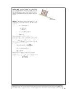
As this composite grade is longer than 4,000 ft (10,000 ft), and part of the curve has a grade of greater than 4%, this grade must be handled using the graphic composite grade methodology illustrated below.

After 2,000 ft of 4% grade, trucks will be traveling at approximately 36 mi/h. This is the speed at which trucks enter the 5,000 ft of 3%. It is as if the trucks had been on the 3% grade for approximately 3,800 ft. Traveling another 5,000 ft along this grade, to 8,800 ft, trucks have re‐accelerated to an approximate speed of 38 mi/h, at which they now enter

the final 3,000 ft of 5% grade. Starting as if they were approximately 1,800 ft along the 5% grade, they travel another 3,000 ft to 4,800 ft. They’re final speed is approximately 28 mi/h, and the composite grade is 5%, 10,000 ft long. (d) As the initial portion of the grade is the steepest, the composite grade is taken to the end of the first segment: 5%, 4,000 ft.

Problem 14-3 A freeway operating is generally rolling terrain has a traffic composition of 12% trucks and 3% RVs. If the observed peak hour volume is 3,200 vph, what is the equivalent volume in pch.

From Table 14.11, for rolling terrain, E T = 2.5 and ER = 2.0. Then: PC Equivalents for Trucks: 3,200*0.12*2.5 = 960 pc/h PC Equivalents for RVs: 3,200*0.03*2.0 = 192 pc/h PC Equivalents for Cars: 3,200*0.85*1.0= 2,720 pc/h Total Equivalent Volume: 3,872 pc/h

Problem 14-3 It is necessary to determine the free-flow speed of the subject freeway using Eqn 14-5: FFS = 75.4 - fLW - fLC – 3.22TRD

0.84

Where:

fLW = 1.9 mi/h (Table 14.5, 11‐ft lanes) fLC = 0.8 mi/h (Table 14.6, 2‐ft clearance, 4‐lane freeway) TRD = 4.2 ramps/mi (given)

FFS = 75.4 – 1.9 – 0.8 – 3.22(4.2

0.84

) = 62.0 mph

From 14.10, the 60-mi/h speed-flow relationship is used for this freeway. Service flow rate are computed using Eqn 14-2; service volumes are computed using Eqn 14-3:

Maximum service flow rates (MSF) are selected from Table 14.3 for a FFS of 60 mi/h: LOS A – 660 pc/h/ln; LOS B – 1,080 pc/h/ln; LOS C – 1,560 pc/h/ln; LOS D – 2,010 pc/h/ln; LOS E - 2,300 pc/h/ln. The heavy vehicle factor is based upon passenger car equivalents for trucks on a 4% grade of 1.5 miles. The pce values are different for the upgrade and the downgrade. ET (upgrade) = 3.75 (Table 14.12, 4% grade, 1.5 mi, 3% trucks interpolated) ET (dngrade) = 1.50 (Table 14.14, 4% grade, < 4mi, 3% trucks extrapolated) Then, using Eqn 14.9:

The PHF is given as 0.92, there are 4 lanes in each direction on the freeway, and the driver population adjustment factor (fp) is 1.00 for a normal driver population. Equations 14‐2 and 14‐3 are implemented in the spreadsheet table shown below.

Problem 14-6 An existing six-lane divided multi-lane highway with a fieldmeasured free-flow sped of 45 mph serves a peak hour volume of 4,000 vph with 12% trucks and no RVs. The PHF is 0.88. The highway has rolling terrain. What is the likely level of service for this section?

To determine the probable LOS for this existing 6‐lane multilane highway with FFS = 45 mi/h, the equivalent ideal lane flow must be determined using Eqn 14‐1:

Where:

V = 4,000 veh/h (given) PHF = 0.88 (given) N = 3 lanes (given) fp = 1.00 (normal driver population assumed)

Then: ET = 2.5 (Table 14.11, Rolling Terrain)

And:

Then

Comparing this to the MSF values of Table 14.4 for a FFS of 45 mi/h, it is seen that the LOS is E.

Problem 14-7 A long section of suburban freeway is to be designed on a level terrain. A level section of 5 miles is however, followed by a 5% grade, 2.0 mi in length. If the DDHV is 2,500 veh/h with 10% trucks and 2% RV’s, how many lanes will be needed on the: a) Upgrade b)Downgrade c) Level Terrain To provide for a minimum level of service of C? Assume that the base conditions of a width and lateral clearance exist and that ramp density is 0.50/mi. The PHF is 0.92.

This is a design application for a section of freeway that goes from level terrain to a sustained 5%, 2‐mile grade. LOS C is the design target. The number of lanes needed to provide this on the (a) upgrade, (b) downgrade, and (c) level terrain is needed. Equation 14‐4 is used:

The FFS of the facility is needed to begin: FFS = 75.4 - fLW - fLC – 3.22TRD

0.84

Where:

fLW = 0.0 mi/h (Table 14.5, 12‐ft lanes) fLC = 0.0 mi/h (Table 14.6, 2‐ft clearance, 6‐lane freeway) TRD = 0.5 ramps/mi (given)

FFS = 75.4 – 0.0 – 0.0 – 3.22(0.5 DDHV MSFC PHF fp

= = =

0.84

) = 73.6 mph =>75 mph

2,500 veh/h (given) = 1,750 pc/h/ln (Table 14.3, FFS = 75 mi/h) 0.92 (given) 1.00 (normal driver population assumed)

There may be as many as three different heavy vehicle adjustment factors for the three segments to be analyzed. They are based upon the appropriate passenger car equivalents for trucks and RVs. Level terrain values are selected from Table 14.11; upgrade (5%, 2 mi) values are selected from Table 14.12 for trucks and 14.13 for RVs; downgrade values are selected from Table 14.14 for trucks and Table 14.11 for RVs (level terrain assumed for downgrade). The resulting values are shown in the table that follows:

The downgrade value for the 2% RVs :As per page 298. The pce’s for RV’s on downgrade sections is taken to be the same as that for level terrain sections, or

1.2.

Problem 14-8 An old urban four-lane freeway has the following characteristics: a) 11-ft lanes d) 7% trucks, no RVs b) No lateral clearances (0 ft.) e) PHF - .90 c) A ramp density of 4.5 /mi f) Rolling Terrain

The present peak hour demand on the facility is 2,100 vph, and anticipated growth expected to be 3% per year. What is the present level of service expected? What is the expected level of service in 5 years? 10 years? 20 years? to avoid breakdown (LOSF) when will it substantial improvements be needed to this facility or alternative routes? This question concerns an old freeway with projected traffic growth in the future. It asks for an evaluation of LOS at various future time‐ points. The easiest way to approach this problem is to create a table of service volumes for the freeway which can be matched against future demand levels. It is first necessary to estimate the FFS of the freeway using Eqn 14‐5: FFS = 75.4 - fLW - fLC – 3.22TRD Where:

0.84

fLW = 1.9 mi/h (Table 14.5, 11‐ft lanes) fLC = 3.6 mi/h (Table 14.6, 0‐ft clearance, 2 lanes) TRD = 4.5 ramps/mi (given)

FFS = 75.4 – 1.9 – 3.6 – 3.22(4.5

0.84

) = 58.5 mph => SAY 60mph

However, this could have been solved either graphically or algebraically as follows:

Where:

V = 2,100 veh/h (given) PHF = 0.90 (given) N = 2 lanes (given) fp = 1.00 (normal driver population assumed) ET = 2.5 (table 14.11, rolling terrain), yielding = fHV = 1/ [1+0.07(2.5‐1)] = 0.905

Thus, Vp = 1289 vph 14.2 => LOS C

D = V 1289/58.5 = 22.03 pc/h/l As per Table S

Or go to figure 14.2, plot 1289 vs FFS curve of 60 results in the LOS C Density Zone Do the same with the adjusted V for the 5, 10 & 20 year growth factor and the results will be the same as above. e.g. at 1) year V = 2822 then Vp = 1732 D.

1732/58.5 = 29.6 pc/h/l LOS